How to Count cells that are not blank using Countif?
The COUNTIF function is a widely-used tool for counting cells that are not empty. It is compatible with various spreadsheet applications, such as Excel, Google Sheets, and Numbers.
![]()
This versatile function can count various formats, such as dates, numbers, text values, blanks, non-blanks, and can perform lookups, including cells containing specific characters. Basically, COUNTIF adds-up the number of cells that satisfy a specified basis.
In this article, we will explore how to use the COUNTIF function to identify non-empty cells, also commonly known as the Not Blank criteria. When applied, the function counts cells with data and disregards those that are empty.
Formula of COUNTIF
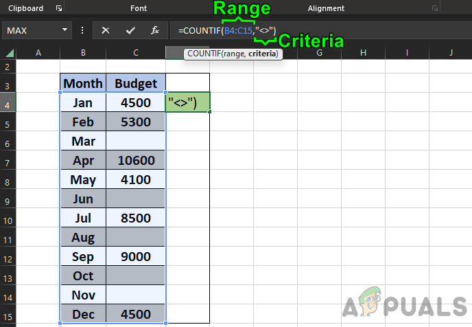
The fundamental formula of COUNTIF requires assigning a range and a criterion. The formula effectively filters cells based on the declared criterion.
=COUNTIF(range, criteria)
Countif Using Not Blank Annotation
Here is the generic syntax for the COUNTIF formula combined with the not blank criteria:
=COUNTIF(range,"<>")
This formula instructs COUNTIF to count all the cells in a specific range that are not empty—indicated by the <> symbol.
Example #1: Single Column
Here is a visual containing two columns labeled Month and Budget. To count the populated cells in the Budget column (C4 to C15), use the following formula:
=COUNTIF(C4:C15,"<>")
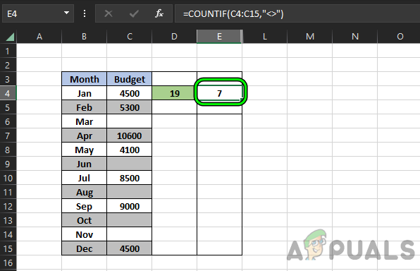
The result, 7, indicates that there are seven cells with content within the specified range.
Example #2: Multiple Columns
To count the non-empty cells in multiple columns (specifically B4 to C15), you should use this formula:
=COUNTIF(B4:C15,"<>")
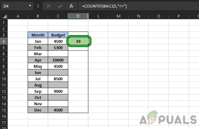
This will produce a result of 19, indicating 19 non-empty cells within the chosen range.
Introducing the COUNTA Function
There exists an alternative to COUNTIF for counting non-empty cells:
=COUNTA(B4:C15)
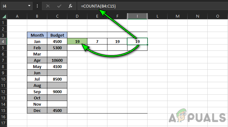
It shows the same result of 19 as the COUNTIF Not Blank function did.
Keep in mind that COUNTA cannot handle more than one argument. If additional criteria are necessary, COUNTIF is the more suitable choice.
The Benefit of COUNTA: Multiple Ranges
COUNTA has an advantage over COUNTIF in that it can handle multiple ranges. As an example, to count non-empty cells across several ranges, COUNTA is quite useful:
By entering this formula into cell I5:
=COUNTA(B4:C15,D4:H5)
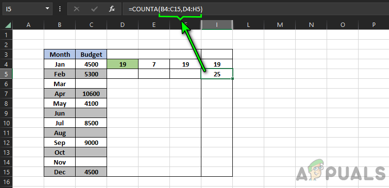
You will come up with a total figure of 25 which spans the two distinct ranges of B4:C15 and D4:H5.
Using COUNTIF for Multiple Ranges and Criteria
While COUNTIF can be applied to multiple ranges, the process is slightly more complex compared to COUNTA.
For instance, observe the following formula in column J4:
=COUNTIFS(B4:B15,"<>",C4:C15,"<10000")
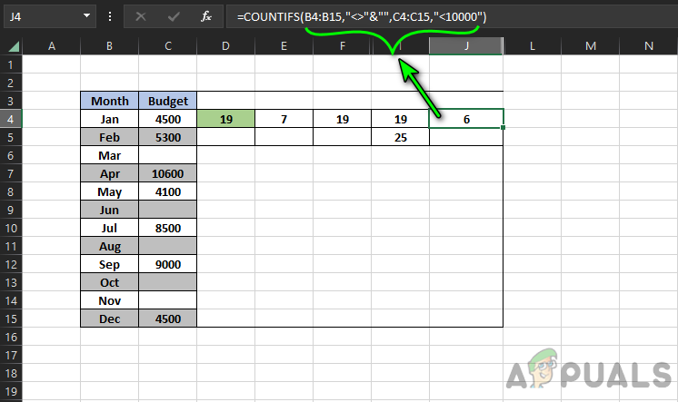
This formula tabulates cells within the specified ranges that are not blank and under 10,000, which totals to 6. If you want to exclude zeroes when counting non-blank cells, the following formula would be suitable:
=COUNTIFS(A1:A10,"<>0",A1:A10,"<>")
To count non-empty cells adjacent to a specific cell, you could use:
=COUNTIFS(A:A,"B",B:B,">0")
Recall that COUNTIFS only counts values that meet all specified criteria. Alternatively, the DCOUNTA function can calculate non-blank cells in a field based on specified criteria.
Use Multiple COUNTIF Functions
If COUNTIFS seems too challenging or unsuitable, using multiple COUNTIF functions can be a workaround. Consider the formula below:
=(COUNTIF(B4:B15,"<>")+COUNTIF(C4:C15,"<>")+COUNTIF(D4:D15,"<>"))
This formula determines all non-blank cells across three distinct ranges. Different criteria can be used for each COUNTIF function if needed.
Problem 1: The Invisible Non-Blank Cells
A complication with COUNTIF, COUNTIFS, and COUNTA functions is that they count cells with spaces, empty strings, or apostrophes (‘), even though these aren’t visible. As a result, the count might be incorrect, leading to incorrect data analysis.
Consider the example below:
=COUNTIF(B4:C15,"<>")
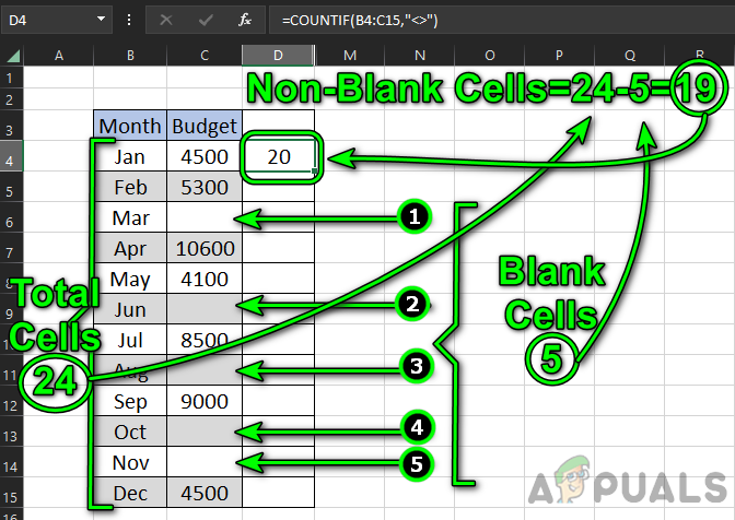
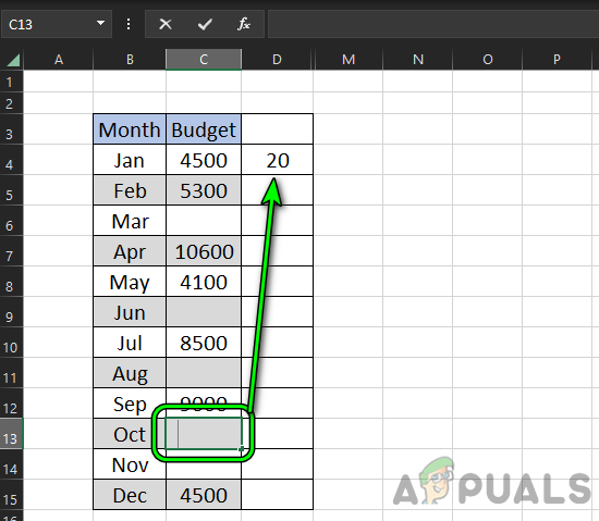
In the demonstrative image, there are 24 cells within B4:C15. Of these, 5 (C6, C9, C11, C13, and C14) are visibly empty. Thus, there should logically be 19 non-blank cells. However, the result in cell D4 reads 20.
It is because cell C13 contains an invisible space, incorrectly included in the count.
Step 1: Identify Invisible Non-Blank Cells with the ‘LEN’ Formula
In the above mentioned scenario, cell C13 shelters a space character.
- This can be detected with the LEN formula. Following the prior illustration, input this formula into D4:
=LEN(C4)
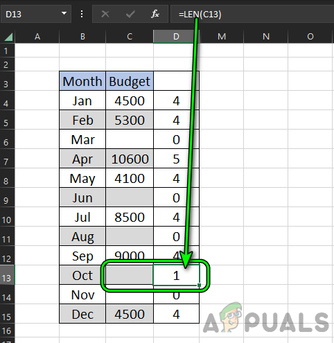
Finding the Cell With a Space by Using the LEN Formula - After you replicate the formula down to D15, you’ll notice cell D13 displays 1 character, suggesting an invisible character exists in C13.
- Upon selecting and deleting the contents of cell C13, you’ll see the count of non-blank cells in D4 correctly displays 19.
Step 2: Verify the Non-Blank Cell Count
To confirm the total count of non-blank cells, arrange the number of empty cells and compare it against the total number of cells in the dataset.
- Use this formula to count empty cells:
=COUNTIF(B4:C15,"")
- This renders a count of 5 in cell G4. The formula =COUNTBLANK(B4:C15) is also valid.
- Next, determine the total number of cells within B4:C15:
=ROWS(B4:C15)*COLUMNS(B4:C15)
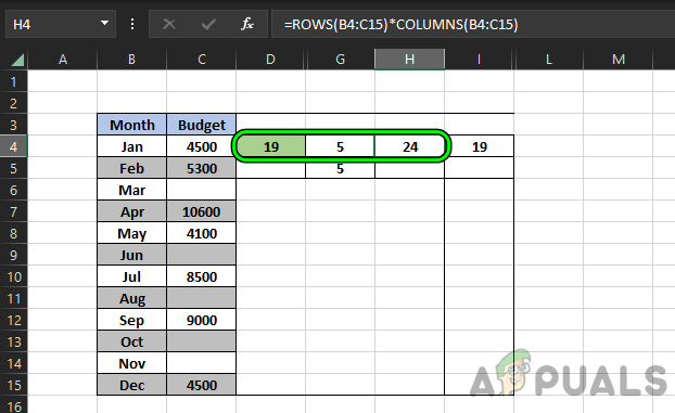
Confirming the Countif Not Blank Result - This shows a total of 24 as indicated in cell H4.
- Hence, we confirm that the COUNTIF ‘Not Blank’ function is correct in reporting 19 non-blank cells.
24 - 5 = 19
Problem 2: The Hidden Apostrophe Problem
Similar to cells containing spaces, a hidden apostrophe can also be problematic as it does not display in the cell’s content and is not considered as a character by the LEN function. Yet, COUNTIF counts cells with a hidden apostrophe as non-blank, which can lead to inaccurate results.
Consider this formula in cell D4 as an example:
=COUNTIF(B4:C15,"<>")
The count shows 20 non-empty cells, which contradicts our earlier understanding that there are only 19 cells that are not blank.
If we apply the LEN function, we’ll discover that it indicates 0 characters for all apparently blank cells.
Solution: Multiply by 1 to Expose the Hidden Apostrophe
To detect a hidden apostrophe, which is usually stored as a text value, you can attempt to multiply the cell’s content by 1. This operation will result in a value error when there is a text value in the cell.
- Enter the following formula in cell F4:
=C4*1
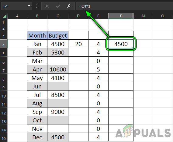
Set a Multiply by 1 Formula in F4 Cell - Now, copy this formula down to cell F15. Notice a #VALUE! error appears in cell F9.
- Select cell C9 now, and observe a hidden apostrophe in the formula bar.
- After deleting it, the result in cell D4 will update and rightfully display the number 19, which aligns with our previous conclusion.
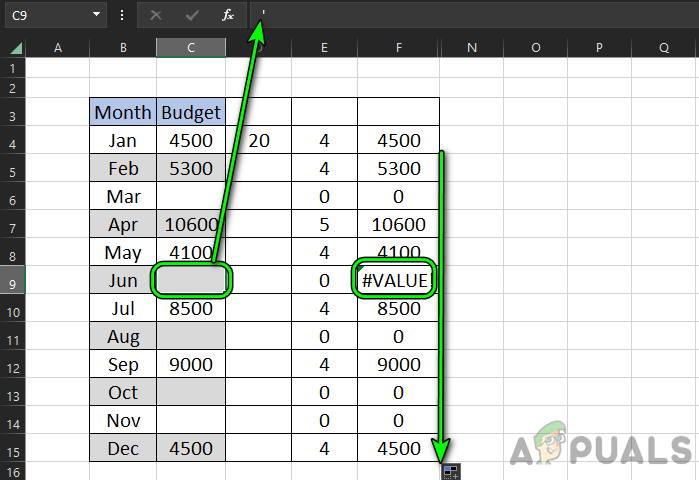
Copy the Multiply by 1 Formula to Other Cells and Value Error Due to Apostrophe in C9 Cell
Problem 3: The Empty String (=””) Issue
Like spaces and apostrophes, empty strings, represented by “=“, can be present in cells without being visible. Although the LEN function does not count an empty string as a character, the Multiply by 1 method, as discussed earlier, effectively detects them.
To illustrate this problem, insert the following in cell C14:
=""
Notice that now the COUNTIF function’s count of non-blank cells has increased by 1, becoming 20, while cell C14 visually appears blank.
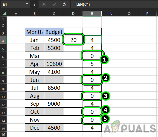
Input this in cell E4:
=LEN(C4)
Copy this formula to E15, and notice that cell E14 shows zero characters, indicating it does not recognize the presence of an empty string, yet COUNTIF counts it as non-blank.
Solution: Use Multiply by 1 to Find the Empty String
- Input the following formula in cell F4:
=C4*1 - Copy this formula down to cell F15 and you will immediately notice a #VALUE! error in the F14 cell.
- This indicates the presence of an empty string in cell C14. After clearing this string, the COUNTIF Not Blank result in cell D4 will accurately return the count of 19.
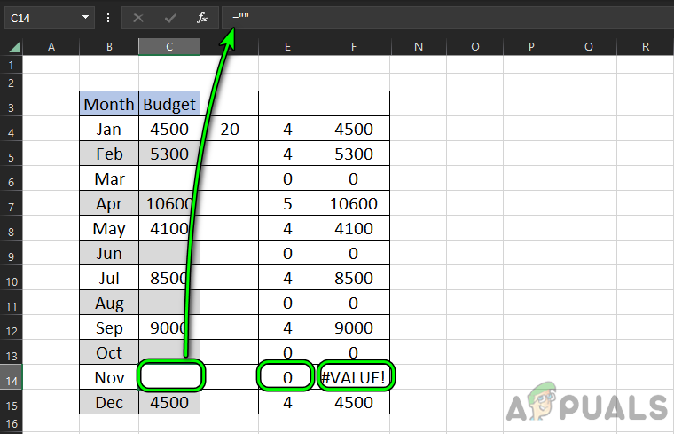
Finding Empty String Cell by Multiplying by 1 Formula
Note: The Multiply by 1 method can also be used to identify cells possessing spaces.
Workaround for All Problems: Using SUMPRODUCT
While the previously mentioned methods to resolve data inconsistencies are effective, they may be impractical when dealing with large datasets. In the example that follows, we face the same issues as before with hidden values such as empty strings and hidden apostrophes in cells.
- To bypass this manual process, consider entering the following formula in cell F4 which employs the SUMPRODUCT function:
=SUMPRODUCT((TRIM(B4:C15)<>"")*1)
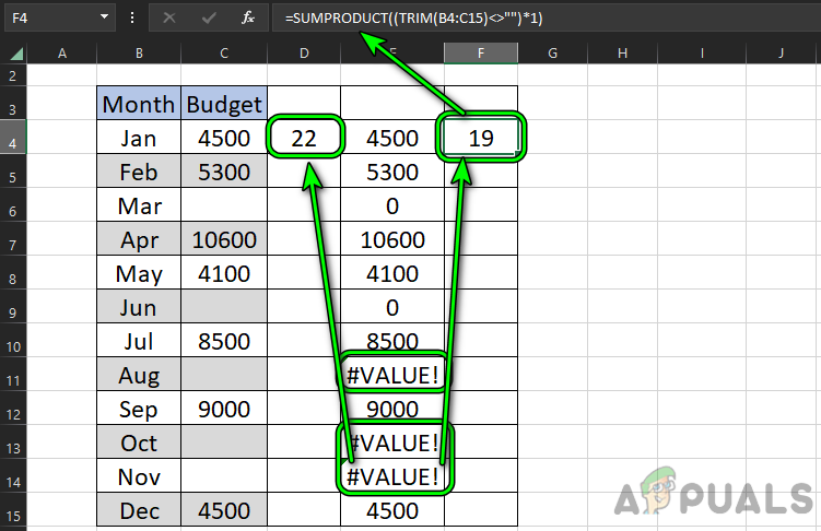
Sumproduct Function Showing the Correct Answer While Countif Not Blank Showing Incorrect Result Due to Invisible Non-Blank Cells - Now, the result in F4 reveals the correct count of non-blank cells which is 19, aligning with our earlier findings.
- The function TRIM(B4:C15) is used to eliminate any leading or trailing spaces from cells.
- The condition TRIM(B4:C15)<>”” singles out cells that are not empty.
- By multiplying the result of (TRIM(B4:C15)<>””) by 1, we transform the Boolean output (True for not empty, False for empty) into numerical values (1 for True, 0 for False).
- The SUMPRODUCT function then multiplies and adds these array values, ultimately providing the sum.
If these methods do not meet your needs, you may consider converting your data into a more structured format, such as a table, which can facilitate the use of structured formulas to count non-blank cells more efficiently.