How to Trace Excel Errors

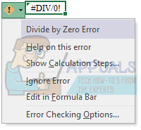
Regardless of the version of excel you are using, there will always be error messages if something is not quite right. All errors presented by excel are preceded by a (#) hashtag and will look like the provided screen shot. Errors will always be shown with a red triangle in the upper left corner of a cell with the particular error message as the cell value.

Types of Errors

There are many types of errors within Excel and it is important to understand the differences between them and why they occur. Below are some error values, what they mean and what they are generally caused from.

#DIV/0 – The #DIV/0 error will occur when the division operation in your formula is referring to an argument that contains a 0 or is blank.

#N/A – The #N/A error is, in fact, not really an error. This more so indicates the unavailability of a necessary value. The #N/A error can be manually thrown using =NA(). Some formulas will throw the error message as well.

#NAME? – The #NAME? error is saying that excel can’t find or recognize the provided name in the formula. Most often this error will appear when your formulas contain unspecified name-elements. Usually these would be named ranges or tables that don’t exist. This is mostly caused by misspellings or incorrect use of quotations.

#NULL! – Spaces in excel indicate intersections. It’s because of this that an error will occur if you use a space instead of a comma (union operator) between ranges used in function arguments. Most of the time you will see this occur when you specify an intersection of two cell ranges, but the intersection never actually occurs.

#NUM! – Although there are many circumstances the #NUM! error can appear, it is generally produced by an invalid argument in an Excel function or formula. Usually one that produces a number that is either too large or too small and cannot be represented in the worksheet.

#REF! – Commonly referred to as “reference”, #REF! errors can be attributed to any formulas or functions that reference other cells. Formulas like VLOOKUP() can throw the #REF! error if you delete a cell that is referred to by a formula or possibly paste over the cells that are being referred too.

#VALUE! – Whenever you see a #VALUE! error, there is usually an incorrect argument or the incorrect operator is being used. This is commonly seen with “text” being passed to a function or formula as an argument when a number is expected.

Error Tracing

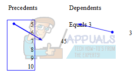
Excel has various features to assist you in figuring out the location of your errors. For this section, we are going to talk about Tracing errors. On the Formulas tab in the “Formula Auditing” section you will see “Trace Precedents” and “Trace Dependents”.

In order to use these, you first have to activate a cell containing a formula. Once the cell is active, select one of the trace options to assist you in resolving your issue. Tracing dependents shows all cells that the active cell is influencing whereas Tracing precedents shows all cells whose values influence the calculation of the active cell.

The Error Alert

When formulas don’t work as we expect them to Excel helps us out by providing a green triangle indicator in the top left corner of a cell. An “alert options button” will appear to the left of this cell when you activate it.

When hovering over the button, a ScreenTip will appear with a short description of the error value. In this same vicinity, a drop-down will be presented with the available options:

1. Help on this error: This will open Excel’s help window and provide information pertaining to the error value and give suggestions and examples on how to resolve the issue.
2. Show Calculation Steps: This will open the “Evaluate Formula” dialog box, also found on the Formulas Tab. This will walk you through each step of the calculation showing you the result of each computation.
3. Ignore Error: Bypasses all error checking for the activated cell and removes the error notification triangle.
4. Edit in Formula Bar: This will active “Edit Mode” moving your insertion point to the end of your formula on the “Formula Bar”.
5. Error Checking Options: This will open Excels default options for error checking and handling. Here you can modify the way Excel handles various errors.

Additional Error Handling

Although the above error handling features of Excel are nice, depending on your level this may not be enough. For instance, say you have a large project where you are referencing various data sources of information that is populated by multiple members of your team. It is likely that not all members are going to input the data the exact same all the time. This is when advanced error handling within Excel comes in handy.

There are a few different ways to handle errors. IFERROR() is a valuable formula providing you two different processes depending on an error being present or not. Other options are using formula combinations such as IF(ISNUMBER()). Most of the time this formula combination is used with SEARCH(). We know that when Excel returns something TRUE it can be represented by a 1. So, when you write =IF(ISNUMBER(SEARCH(“Hello”,A2)),TRUE,FALSE) you are saying, “If you find Hello in A2 return a 1, otherwise return a 0.”  Another formula that comes in handy for later versions of Excel is the AGGREGATE() function. We’re going to go over some brief examples below.

Generating an error without the use of IFERROR()

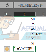
1. In the below example you will see that we are trying to subtract “text” from the sum of another range. This could have occurred for various reasons but subtracting “text” from a number obviously will not work too well.
2. In this example it generates a #VALUE! error because the formula is looking for a number but it is receiving text instead
   
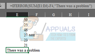
3. In the same example, lets use the IFERROR() and have the function display “There was a problem”
4. You can see below that we wrapped the formula in the IFERROR() function and provided a value to show. This is a basic example but you can be creative and come up with many ways to handle the error from this point forward depending on the scope of the formula and how complex it may be.

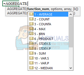
Using the AGGREGATE() function can be a little daunting if you have never used it before.

1. This formula is however versatile and flexible and is a great option for error handling depending on what your formulas are doing.
2. The first argument in the AGGREGATE() function is the formula you want to use such as SUM(), COUNT() and a few others as you see in the list.
   
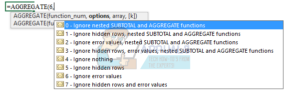
3. The second part of the argument are options in which you can incorporate with the formula in the first argument. For the sake of this example and this lesson, you would select option 6, “Ignore error values”.
   
4. Lastly you would simply but the range or cell reference that the formula is to be used for. An AGGREGATE() function will look similar to this:
   =AGGREGATE(2,6,A2:A6)
5. In this example we are wanting to COUNT A2 through A6 and ignore any errors that may occur
6. To write the example formula as a different method it would look like this:
   =IFERROR(COUNT(A2:A6),””)

So as you can see there are many options and ways to handle errors within Excel. There are options for very basic methods such as using the Calculation Steps to assist you or more advanced options like using the AGGREGATE function or combining formulas to handle various circumstances.

I encourage you to play around with the formulas and see what works best for your situation and your style.