How to Use the SUM Function in Google Sheets
Google Sheets can be used to keep your work organized. With a few formulas, you can work with sheets very easily that will help you make your working time shorter, and help you save a lot of time. While it might take you a lot of time to manually calculate the total for a row or column, you can always use formulas on Google Sheets to find the sum of a certain row or column.
The Function for SUM in Google Sheets
=SUM(NUMBER_1,NUMBER 2)
OR
=SUM( CELL NAME1: CELL NAME2)
When using the SUM function on Google Sheets, you need to make sure that you are writing the correct numbers that you want to be added or totaled. I would suggest that you add the cell numbers instead of adding the numbers as it will automatically get altered in case you make any changes to the original numbers.
If there are two or more specific cells in a row or column that you want to be added, you will use the first format for the SUM function which is mentioned above. You will separate each number, or cell name with a comma and end the function with a bracket. This will eventually give you a total for the specific cell names that you have entered.
For example, if you want to add cell A1,A4, and A6, this is how you will write the formula:
=SUM(A1,A4,A6)
You can always write the number in the cells that you want to add. But, writing the cell name in the SUM function would be a better idea for future adjustments in the document. If you write the number and not the cell name, you will have to manually change the numbers in the function if any changes are required for the original cell. But, if you add the cell name, the function will automatically adjust the addition that just took place using the new number added to the cell mentioned in the formula.
The other format for SUM function can be used when you want an entire row or column to be added. Here, you don’t need to separate each number or cell name with a comma. All you need to do it use the colon sign, ‘:’ from your keyboard between the first cells name and the last cells name on the row or column that you want to add. Look at the example below to understand this format better.
=SUM(A1:A6)
This is an easier way to add a column or row on Google Sheets.
A Few Things to Remember When Using Google Sheets
- To add numbers, columns or rows, you need to start the function with ‘=SUM(…’.It is after the bracket open that you add details of the cells you want to add or the numbers that you want to sum up.
- To make your Google Sheet look organized, always highlight the cell that shows the total sum of any set of numbers. This will give a very professional look to your Google Sheets.
How To Use the SUM Function
- Open a Google Sheet with data.
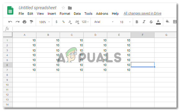
Opening data on Google Sheets - If it is an entire row or column that you need to add, then right after the column or row ends, click on the empty cell that is next, and start writing the SUM function for addition.=SUM(…
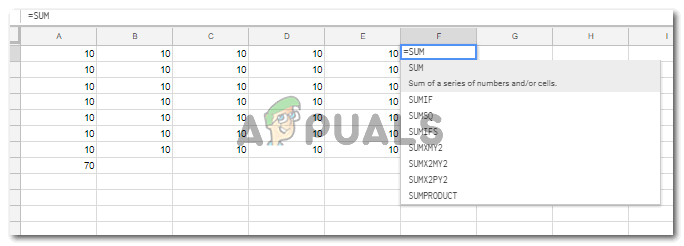
- The minute you add the equals to sign, functions and formulas will start showing right under that cell like a dropdown list which is where you can find the SUM function.
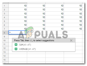
Typing the SUM function - Choose the function from the dropdown list that appears, or, type in the cell the function and the cell numbers that you want to add according to the two formats that I have mentioned above, depending on which numbers you want to add.
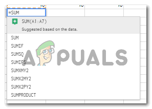
Select the function as it appears in the list below the cell or type it down - Adding the last bracket to the formula shows the answer for this addition like a pop-up right above the cell you added the SUM function to.

The sum for cells will show here - Press the Enter key from your Keyboard, and this will show you the answer in this cell.
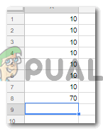
Press Enter to show the sum of numbers in this cell - The same steps could be followed for rows as well.
Follow the same steps for Rows 
Using the colon to add all the cells between the first and the last one on the row 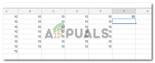
Press Enter
Benefits of Using Cell Name instead of Numbers in the Cell
- Assume that the numbers for cells have been altered.

Changes on the sheet - If you used the Cell name, the answers in the cell where you entered the SUM function will get adjusted automatically.
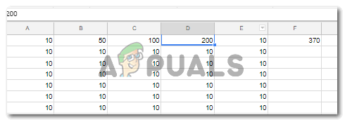
Automatic adjustment in the sum You will not have to manually change this in the SUM function, which would be the case if you add numbers in the SUM function.


