How to Use the ‘Freeze’ Feature of Google Spreadsheet?
Google Spreadsheet is used by many businesses to keep a record of their data. People also use it for personal use. In either way, if the data is too large, and hides the headings for rows and columns every time you move your spreadsheet to the right or down, there are chances you might find difficulties in remembering which row or column has the heading for what part of the data. To avoid this confusion, and to make sure that the data is entered correctly under the same heading even if you are working on cell 1000, you can freeze the rows and columns for headings. This will lock the rows and columns for the headings cells or till the cells you want the rows or columns to be frozen.
How Does Freezing Rows and Columns Help?
Assume that you need to add a data set of 1000 or more companies. Now every time you go down a column after the page on the screen ends, the spreadsheet keeps getting scrolled down, and now you cannot see the headings which were in the first row. This is where freezing the heading cells, or the title rows and columns helps the user, add data on the spreadsheet, making your work much easier.
If you did not have an option to free cells, you would have to go back to the top of the page to make sure which column or row has which data. And in such a case, the user is prone to make huge mistakes in the data entry.
Zero error in the data you enter is one of the most significant advantages of freezing cells in Google Spreadsheet. Since the results of any data, whether it is the total, or answer to a formula is dependent on the value that is entered in the respective cell. And if that value is incorrect, say for example you had to write 20,000 profit value for company A but you wrote it for company B, this will change the results, causing major errors in calculations.
Steps to Freeze a Row or Column on Google Spread Sheet
If you want to freeze a row or a column on Google Spread Sheet, follow the steps as mentioned below. To show how the cells get scrolled down or towards the right, I have used an example for a class, where I have to enter the name of the student, the marks of the students and their total.
- Open your Google Spread Sheet, and enter the data as you like. Format the headings accordingly to make them stand out in comparison to the rest of the text. You can write the headings in bold, a different color or a different font, depending on your nature of work.
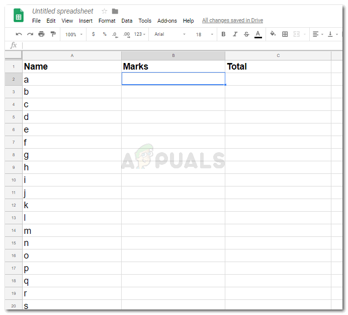
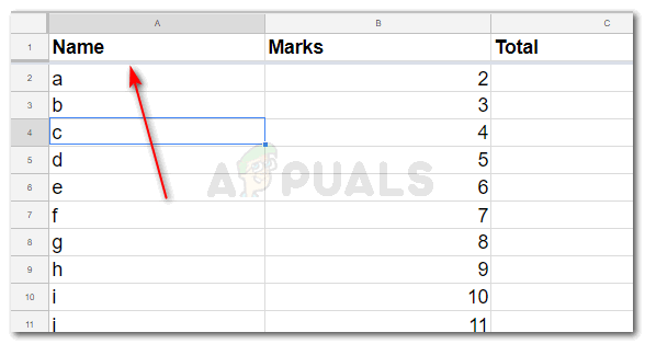
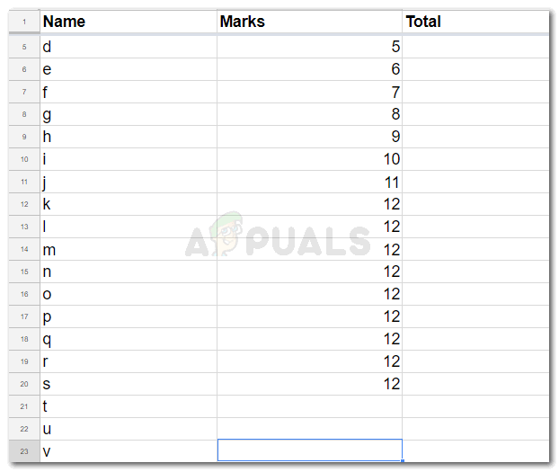
Open Google Sheets and add the headings for your work. You can also open an already existing file. - The image below shows that when I try to add more names or numbers and go down by each column, the headings are not visible on the screen now because the first row is not frozen.
The title rows and columns are not visible - To freeze the first row, or the heading rows. Selection of the first row or column, or cell is not a requirement. You can also freeze these rows and columns without selecting them.
You don’t need to select for the first 2 rows or columns to be frozen - I will click on View which is on the top most tool bar of Google Sheets.
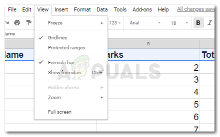
View - Locate the option for ‘Freeze’, which is the very first option under ‘View’. Bring the cursor to it, or click on it to make the extended options to show.
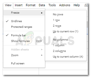
View>Freeze The option for ‘No Rows’ or ‘No Columns’, means that you don’t want any of the rows or columns to be frozen. Whereas the option for 1 row, 2 rows, 1 column or 2 columns will freeze the first or the second row or column, depending on which option you click on.
The next option, which says ‘up to current row’ or up to current column’, for this, you will have to select the row or column, this selection shows that you want all the rows or columns above this point or before this point to be frozen so that you can view the headings or value accordingly. - A grey-ish line appears as soon as you freeze a row or column. This shows that these rows and columns are frozen shown in the images below.
Grey line for frozen row 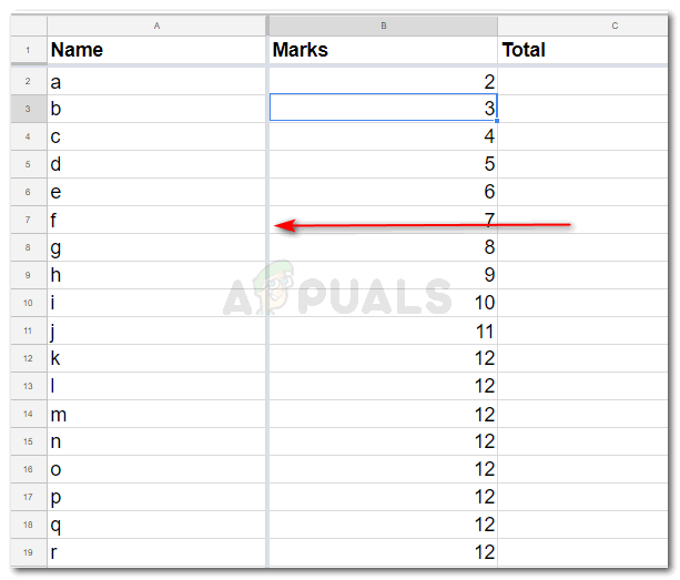
Grey line for the frozen column - Now when you scroll down the page, or move towards the right of the spread sheet, these frozen cells will still appear on the screen even if you are on cell 1000.
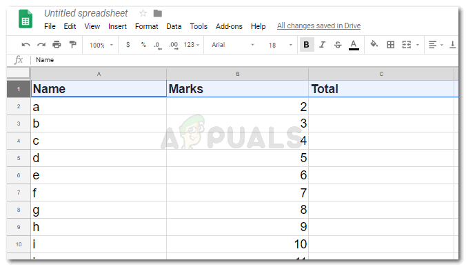
Headings in the first row visible now. 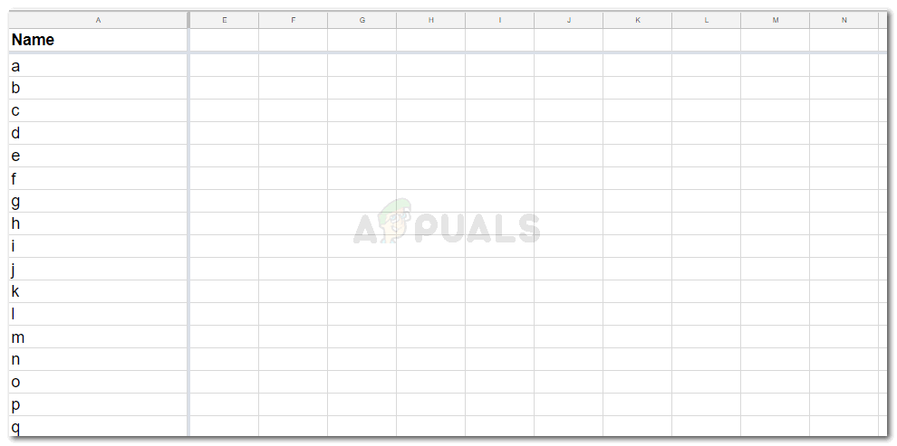
Headings in the first column visible now.
You can try this for yourself on Google Sheets, and notice the ease that you will feel in freezing rows and columns. This could be a lifesaver for people who have a job to analyze, or add data into sheets which are huge in number.