How to Shade Rows and Columns in Microsoft Excel
Microsoft Excel allows the user to shade columns and rows on a worksheet according to the values, and other important determinants in their work. There are two ways in which you can format your cells, columns or rows in an Excel worksheet.
- Conditional Formatting
- Using the MOD formula
Shading the Cells Using Conditional Formatting
Conditional formatting already has a number of ways in which you can alter your cells. These are inbuilt settings for the Microsoft Program, for which you only have to click on the formatting style that you like.
- Open your Excel sheet to a new file, or use the one which already has values in it.
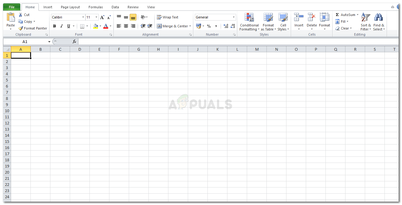
Open Microsoft Excel On the Ribbon for different formatting options for your sheet, you will find the option for Conditional Formatting. But before this, it is highly important that you select the area of cells where you want this formatting to be implemented on.
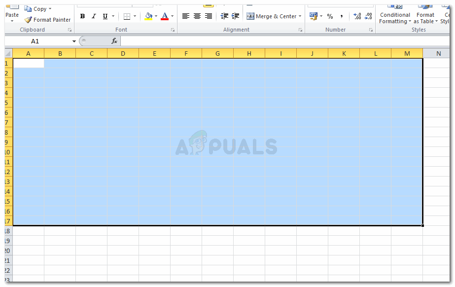
Select the Cells you want to show shaded alternate rows 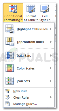
Click on Conditional Formatting Tab on the Ribbon - Highlight cell rule and Top/bottom rules are what determines which cell will be highlighted with a color, depending on the set of values which are a part of your work. Look at the pictures below to view the different options for formatting your cells.
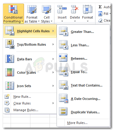
Highlight Cells Rules 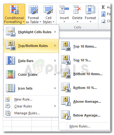
Top/Bottom Rules 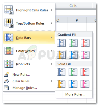
Data Bars 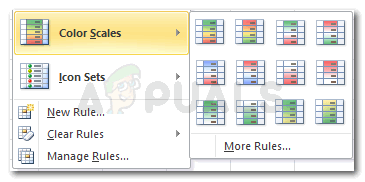
Color Scales 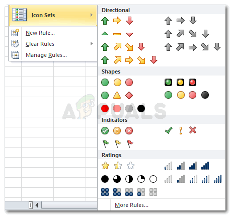
Icon Sets - Now for the first two settings under Conditional Formatting, when you click on any of the options as shown in the image for Highlight Cells Rules and Top/Bottom Rules, a dialogue box appears, where you enter the values for highlighting the cells with those values, values higher than the value you entered, or values lower, equal to or even between a certain bracket will be highlighted, according to your selection.
Adding the numbers as requested by the format you select. This will be different for all the different conditional formats.
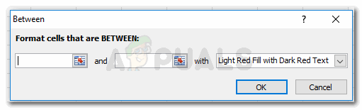
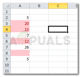
As an example, I selected the option for ‘between…’, and entered a range in the space provided. Now on the worksheet, all the cells which will have a value between this range will get highlighted as shown in the image below.
Shading the Cells Using MOD Formula
- For this again, you need to select the rows/columns that you want to be alternately shaded.
- Click on the Conditional Formatting tab and click on ‘New Rule’, which is the third option from below.An extended window will appear on the screen.
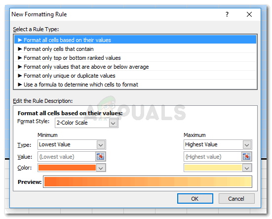
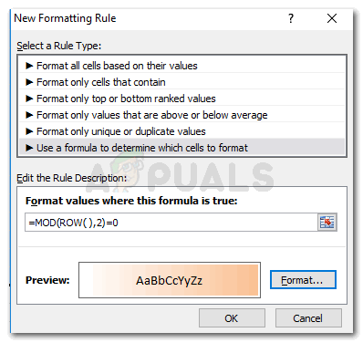
Default settings of Formatting Rules You need to ‘select a rule type’ which says ‘Use a Formula to Determine Which Cells to Format’.
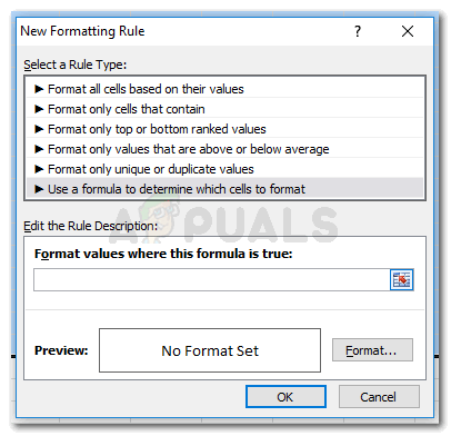
Click on the last one from this list - Enter the MOD formula in the space provided: =MOD(ROW( ),2)=0
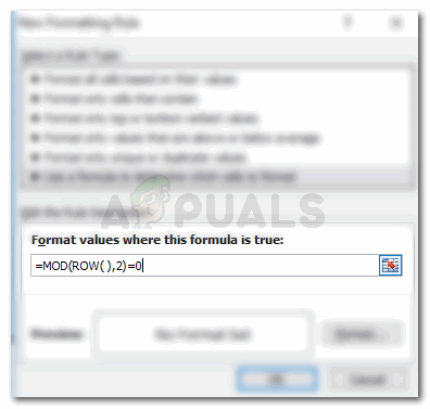
Using the MOD formula here. - Format the cells, select the color and style by clicking on the Format icon right below the space for the formula.
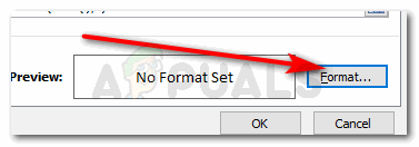
After entering the correct MOD formula, you can edit the format of the color, shading style and more for the cells. 
Select a color and a fill effect to make your work look good. 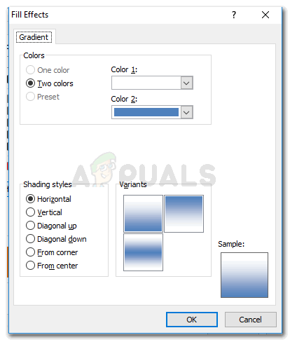
More formatting for the way the cell is shaded 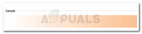
Selecting Vertical shading style - Click OK, and your cells will show alternately shaded rows.
Confirm your settings by clicking OK 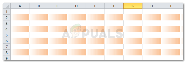
Your Rows have been formatted.
Understanding the MOD Formula
The MOD formula can be very helpful for users and is pretty easy to understand how it works. It is not important that everyone would always want the alternate ‘rows’ to be shaded. Sometimes, people might even want the columns to be shaded and this might not be wanted at alternate gaps. You can always replace the word ‘ROW’ in the formula with ‘COLUMN’, to implement the same formatting on the columns instead. And change the numbers in the formula as well for the gap and beginning settings. This will further be explained below.
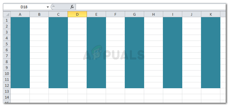
=MOD(COLUMN( ),2)=0
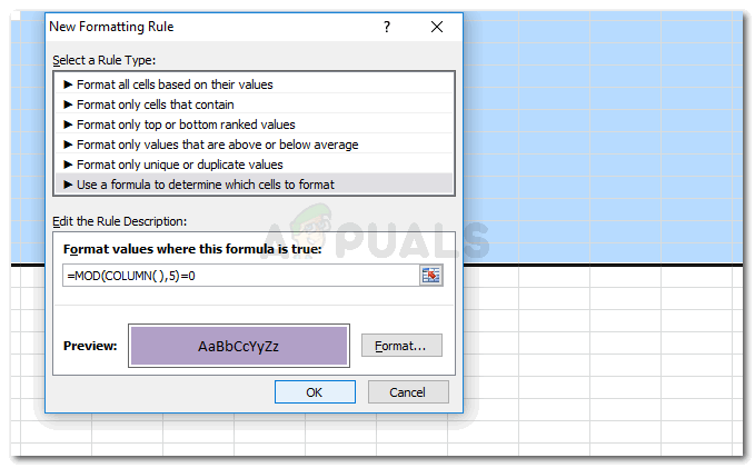

Now, the number 2 here, shows that every second column will be shaded according to the colors that you have selected. But, if you don’t want every second row/column to be shaded, but instead want the fourth or the fifth row/column to be shaded, you will change the number 2 here in the formula to 4 or 5, depending on how many rows/columns gap you want in between.
Similarly, if you want the software to start the shading from the first column, and not from the second, you will change the number 0 in the formula with 1.