How to Round Numbers in Google Sheets Using MROUND Function
Working with Google Sheets can be very easy once you understand the formulas that can be used for various functions. Similarly, to round a number to the nearest decimal place can be done through the ‘MROUND’ function in Google Sheets. All you have to do is follow the formatting of the function, that is, where you need to write which number, and you are good to go. Here is what the MROUND function in Google Sheets looks like:
=MROUND(value, factor)
What Does Value in the MROUND Function Mean?
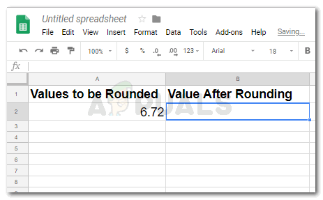
Value is the number that you want to be rounded to the nearest decimal. Say, for example, 6.72, is my value for this example which I will be rounding off to the nearest decimal places in the following examples to make you understand the different decimal places for which you can round these off.
What Does Factor in the MROUND Function Mean?
A factor is basically the number for how many decimal places you want the value you entered on the Google Sheets to be rounded to or the rounded number should be a multiple of that Factor that you just entered. For example, if 6.72 is my value, and if I want the numbers to be rounded to the nearest, say, 0.05, I will write 0.05 in place of ‘factor’ in the MROUND function.
Google Sheets Basics to Remember
- Every formula can only be regulated if you enter the ‘=’ sign. The program will not make the function work if this sign is not added.
- Enter key finalizes the formula and the values entered. So make sure you add the number carefully. However, you can edit the values later as well.
- Brackets are an important part of any formula.
Let’s look at how we can use the MROUND function on Google Sheets through the steps mentioned below.
- Open your Google Sheet, and enter the data that you need to. If it is an answer you need to be rounded, you will add this formula in a cell next to that value or can implement it on the same cell. You are free to choose the cell which you want to show the rounded value. For this example, I will simply show the value and the factors that I add in the MROUND function to help you understand how to use this function.
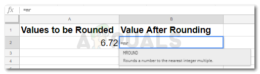
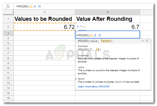
the MROUND for Google Sheets is used to round numbers to the nearest factor added by you. - Start your formula with ‘=’, and write MROUND. The minute you write the M, you will see the function as shown in the picture below, you can simply click on this to make the formula working.
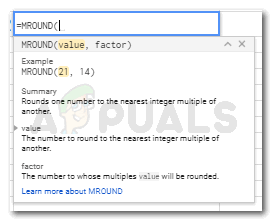
Click on the function MROUND It will also show you how you can enter the values. It explains to its users what the value represents and what the factor represents. This will be a great help for people who don’t understand or find it hard to understand the difference between value and factor.
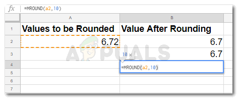
Google Sheets explains the MROUND function once you start typing in the cell after selecting the MROUND function. - Now, you can enter the value (cell number for the where the value has been entered on the Google Sheets), in my case, the cell was A2, yours might be different. And to round it to the nearest multiple of 0.05, I will add 0.05 as the factor. After writing the function, I will press enter which will get me an answer.
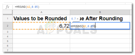
Add the value and the factor for your MROUND function. Make sure you enter the right cell number or the answer for your function will not be accurate. 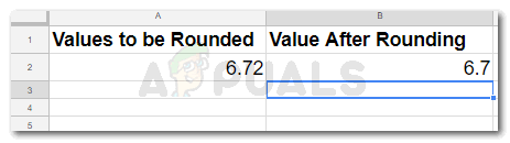
Pressing enter after entering the MROUND function with the correct values will get you an answer. - To round the value to the nearest 0.1, you will write 0.10 or 0.01 in the place for factor in your MROUND and press enter.
Round your numbers to the nearest 0.10 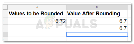
Your value has been rounded to its nearest multiple of 0.10 - You can also round your values to the nearest whole numbers. To round your value to the nearest 5’s, you will have to add the number 5 in your MROUND for space provided for ‘factor’.’
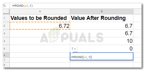
Round your numbers to the nearest 5 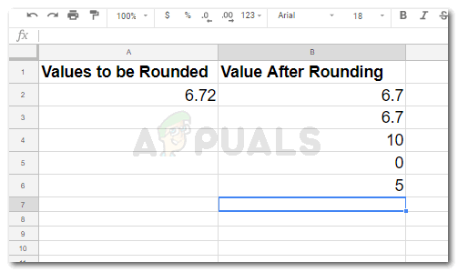
Your answer to the nearest 5 according to your MROUND function. - To round the value in your Google Sheets to the nearest 10’s, you will add this function and these values. Keep in mind that the cell numbers I have used are according to my example. Your cell numbers can vary obviously.
Round your value to the nearest 10. by following the function shown in the image. Make sure you enter the cell number as per your Google Sheet 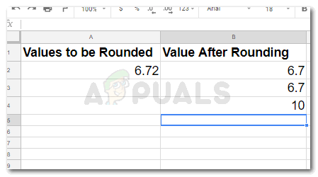
Your answer for rounding values - To round the value that you entered to the nearest 100, you will add ‘100’, in the place for factor in your MROUND as shown in the image below.
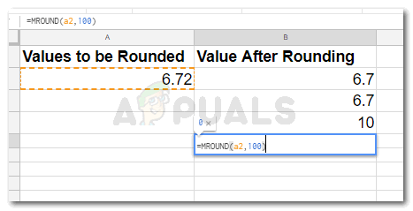
Round your numbers to the nearest 100 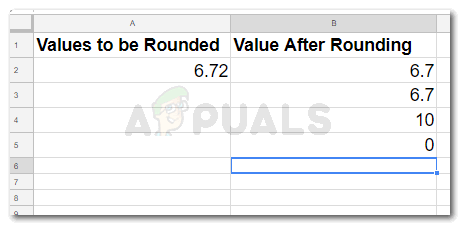
Nearest 100 in this case is 0, since the value is 6.72