How to Multiply on Google Sheets
Working with Google spreadsheets can be very easy if you learn how to add formulas to the cells, which are the basics of using any spreadsheet, whether it is Google or Microsoft office. Here, we are going to learn how to multiply in a Google Spreadsheet. But before we go the main formula or technique to learn this process of multiplying, there are a few things which you must remember when working on a Google Spreadsheet.
If you are applying a formula to a certain cell, you always begin the formula with an ‘equals to’ sign, i.e. ‘=’. If you add the rest of the formula to the cell, say you have to write ‘sum(A5+B%)’, and you forget to add the equals to sign before the word sum, you will not get the expected outcome.
Secondly, when you need to multiply the value in a cell, you use the ‘*’ symbol, which is the asterisk. If you have ever noticed a calculator on the laptop, or in the computers in the past, the calculator never had an ‘x’ for multiplying, but instead had an asterisk which was used as an alternate symbol.
Lastly, the most important thing you need to remember when applying a formula to a cell in Google Spreadsheet is that pressing the enter key after adding the complete formula will bring you the answer to the value you are looking for. Of course, for this, you need to make sure that the formula has the right cells written and the correct words relevant to that formula are used in the current cell where you are adding a formula.
How to Multiply in a Google Spreadsheet?
- Add data to your spreadsheet that you want to be multiplied. Now, adding data could be your first step, however, to apply a formula to a cell does not require you to add the data first. You can add formulas to different cells so that the functions for each cell are pre-decided. I will add the data first for this example and then add the formula.
Using Google Spreadsheets to create a database or for simple assignments 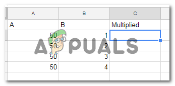
Add the required data as shown in the picture. - Once you have added the data, you will add the equals to sign before adding the cells you want to be multiplied. For example, it is cell A and B that you want to be multiplied, you will write =A*B. Working on a spreadsheet, however, requires the number of the cell as well, so you will write =A2*B2*, just how I have shown in the example below.
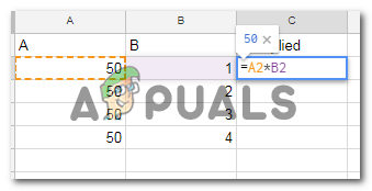
Add the multiplication formula as displayed in the picture to multiply any two cells or more. The asterisk, ‘*’ is the main key for multiplication. Missing the asterisk sign in your formula will not make the cell function like it is supposed to for multiplication. - After writing the complete formula, using the exact number of cells, you are now going to press the enter key on your keyboard. The minute you press enter, a value will appear in the cell where you applied the formula. The correct answer will only appear in the cell if you have added the correct cell alphabet and correct cell number in this current cell. So be careful when adding the formula.
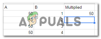
Pressing enter means you have finalized the formula and are good to go. Once you press enter, the value/answer as per the added formula will appear in the cell. - Now for the rest of the cells, you either manually add the formula in each cell, or, you can use a short method to repeat the formula you applied on the first cell of that column or row on the rest of the cells in the same column or row. Now since we have added the formula in the cell C2, we will select this cell and bring the cursor to the edge of this cell, the mouse/ cursor, will change its look and become like a ‘plus +’ sign. Now, to apply the same formula on the rest of the cells under the column C, we will keep the cursor clicked on the right corner of the cell, and keep the mouse pressed, while dragging the mouse slowly down to the last cell till where you have added the data, and want the formula for multiplication to be applied.
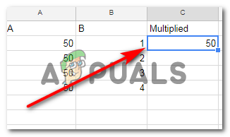
Click on the cell whose formula you want to be copied on the rest of the cells. Clicking on that cell will create these blue borders as shown in the picture. 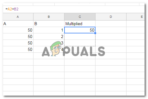
Click and keep the mouse pressed, while simultaneously dragging the cursor down the rest of the cells. 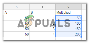
Formula applied All the multiplied values will automatically appear on all the cells that you have covered through the dragging process. This is a much easier method of applying the same formula to all the cells that fall under one column or one specific row. However, if there are different cells for which you want this formula, you will have to add this formula manually.


