4 Ways to Fix: Excel Error ‘An array value could not be found’
Microsoft Excel is a spreadsheet program developed and distributed by Microsoft. It is available across almost all platforms and is used extensively for business and other purposes. Due to it’s easy to use interface and numerous formulas/functions, it has made easy documentation of data a reality. However, quite recently, a lot of reports have been coming in where users are unable to apply a formula to replace a specific letter for a word and an “An Array Value Could not be Found” Error is displayed.
Usually, there are many formulas that can be applied to make entrail certain commands. But users experiencing this error are unable to do so. Therefore, in this article, we will be looking into some reasons due to which this error is triggered and also provide viable methods to fix it.
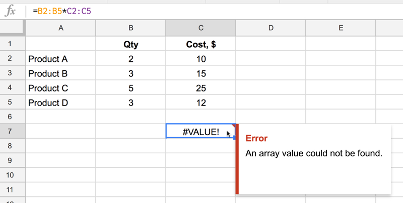
What Causes the “An Array Value Could not be Found” Error on Excel?
After receiving numerous reports from multiple users, we decided to investigate the issue and looked into the reasons due to which it was being triggered. We found the root cause of the issue and listed it below.
- Wrong Formula: This error is caused when the substitution formula is entered incorrectly. Most people use the substitution formula to replace a specific letter with a word or a line. This ends up saving a lot of time but if entered incorrectly this error is returned.
Now that you have a basic understanding of the nature of the problem, we will move on towards the solutions. Make sure to implement these in the specific order in which they are presented to avoid conflict.
Solution 1: Using Substitute Array Formula
If the formula has been entered incorrectly, the substitution function will not work properly. Therefore, in this step, we will be using a different formula to initiate the function. For that:
- Open Excel and launch your spreadsheet to which the formula is to be applied.
- Click on the cell to which you want to apply the formula.
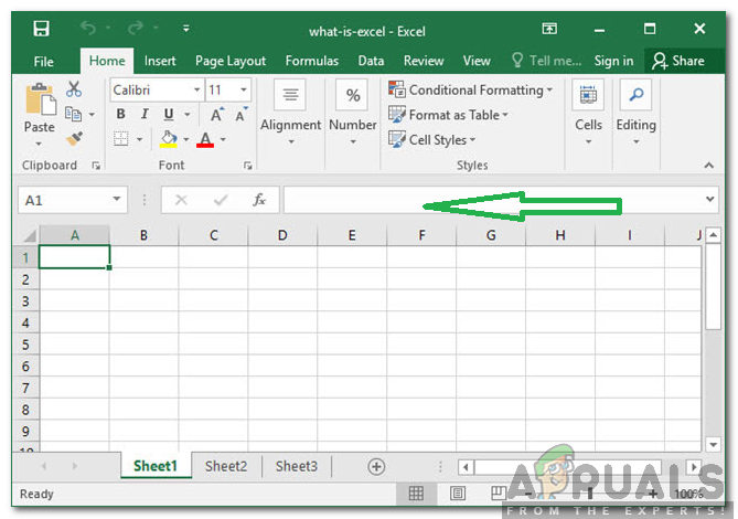
Selecting the cell - Click on the “Formula” bar.
- Type in the following formula and press “Enter”
=ArrayFormula(substitute(substitute(substitute(E2:E5&" "," y "," Y ")," yes "," Y ")," Yes "," Y "))
- In this case, “Y” is being replaced with “Yes“.
- You can edit the formula to fit your needs, place the letter/word that needs to be replaced in place of “Y” and the letter/word that it needs to be replaced with needs to be placed in the place of “yes”. You can also change the address of cells accordingly.
Solution 2: Using the RegExMatch Formula
If the above method didn’t work for you, it is possible that by approaching the problem with a different perspective might solve it. Therefore, in this step, we will be implementing a different formula which uses a different set of commands to get the work done. In order to apply it:
- Open Excel and launch your spreadsheet to which the formula is to be applied.
- Click on the cell to which you want to apply the formula.
- Select the “Formula” bar.
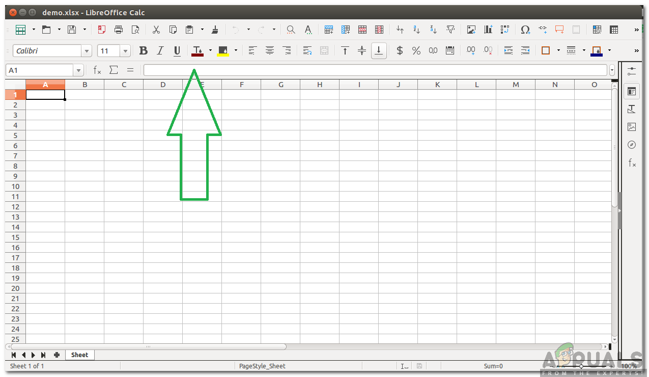
Selecting the formula bar - Enter the formula written below and press “Enter”
=if(REGEXMATCH(E2,"^Yes|yes|Y|y")=true,"Yes") - This also replaced “Y” with “Yes”.
- The values for “Y” and “Yes” can be changed to fit your needs.
Solution 3: Using Combined Formula
In some cases, the combined formula generated from the above mentioned two formulas gets the trick done. Therefore, in this step, we will be using a combined formula to fix the error. In order to do that:
- Open Excel and launch your spreadsheet to which the formula is to be applied.
- Select the cell to which you want to apply the formula.
- Click on the “Formula” bar.
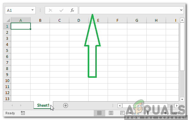
Clicking on the formula bar - Enter the formula mentioned below and press “Enter”
=ArrayFormula(if(REGEXMATCH(E2:E50,"^Yes|yes|Y|y")=true,"Yes")) - This replaces “Y” with “Yes” as well and can be configured to fit your conditions accordingly.
Solution 4: Using RegExReplace Formula
It is possible that the “RegExReplace” formula might be required to eradicate the error. Therefore, in this step, we will be using the “RegExReplace” formula in order to get rid of the error. For that:
- Open Excel and launch your spreadsheet to which the formula is to be applied.
- Select the cell to which you want to apply the formula.
- Click on the “Formula” bar.
Clicking on the Formula bar - Enter the formula mentioned below and press “Enter”
=ArrayFormula(regexreplace(" "&E2:E50&" "," y | yes | Yes "," Y ")) - This replaces “Y” with “Yes” and can be configured to fit your situation accordingly.