How to Create Reports in Microsoft Excel
All the people working in a professional environment understand the need to create a report. It summarizes the whole data of your work or the company’s in a very accurate manner. You can create a report of the data you entered on an Excel Sheet by adding a PivotTable for your entries. A Pivot table is a very useful tool as it calculates the total for your data automatically and helps you analyse your data with different series. You can use a PivotTable to summarize your data and present it to the concerned parties as a report.
Here is how you can make a PivotTable on MS Excel.
- It is easier to make a report on your Excel sheet when it has the data . After the data has been added, you will have to select the columns or rows you want a PivotTable for.
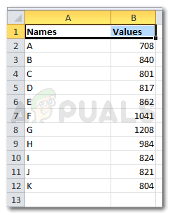
add the data 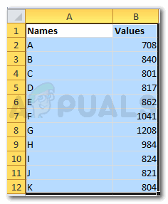
Selecting the rows and columns for your data - Once the data has been selected, go to Insert that is showing on the top tool bar on your Excel software.
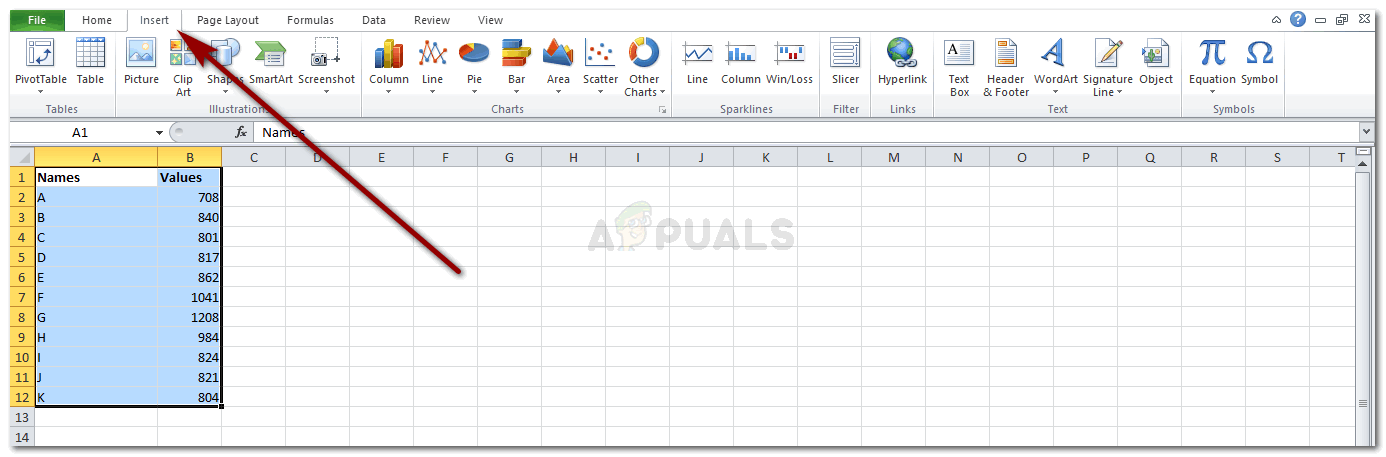
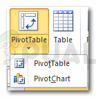
Insert Clicking on Insert will direct you to many options for tables and other important features. On the extreme left, you will find the tab for ‘PivotTable’ with a downward arrow.
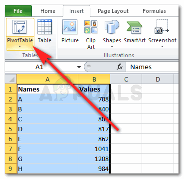
Locate PivotTable on your screen - Clicking on the downward arrow will show you two options to choose from. PivotTable or PivotChart. Now it is up to you and your requirements what you want to make a part of your report. You can try both to see which one looks more professional.
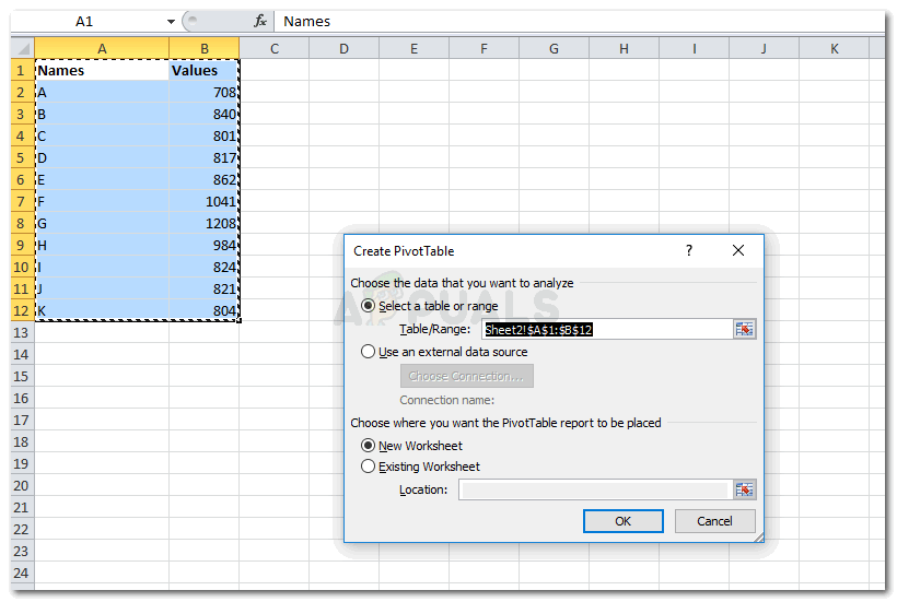
PivotTable to make a report - Clicking on PivotTable will lead you to a dialogue box where you can edit the range of your data, and other choices of whether you want the PivotTable on the same worksheet or you want it on a completely new one. You can also use an external data source if you don’t have any data on your excel. This means, having data on your Excel is not a condition for PivotTable.
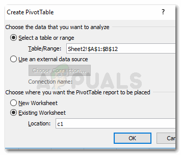
selecting the data and clicking on PivotTable You need to add a location if you want the table to appear on the same worksheet. I wrote c1, you can choose the middle of your sheet as well to keep it all organized.
PivotTable: selection of data and location - When you click on OK, your table will not appear as yet. You need to select the fields from the field list provided on the right of your screen just as shown in the picture below.
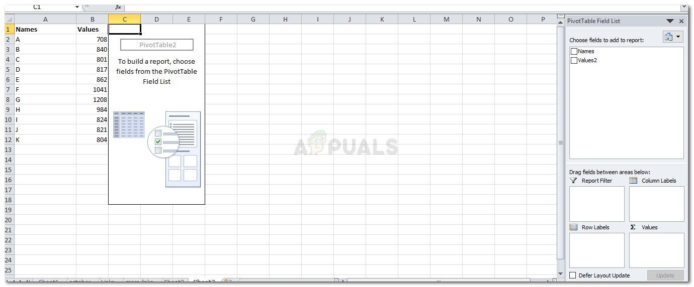
Your report still needs to go through another set of options to finally be made - Check either of the two options for which you want a PivotTable for.
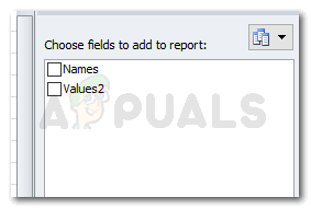
Check the field you want to show on your report You can choose one of them, or both of them. You decide.
- This is how your PivotTable will look like when you choose both.
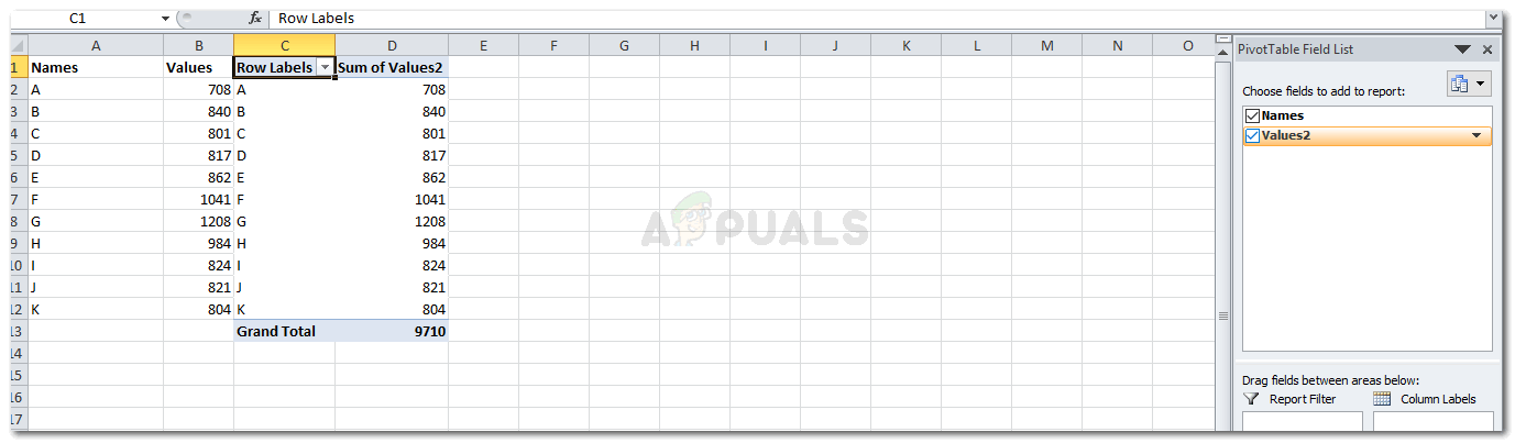
Displaying both the fields And when you select one of the fields, this is how your table will appear.
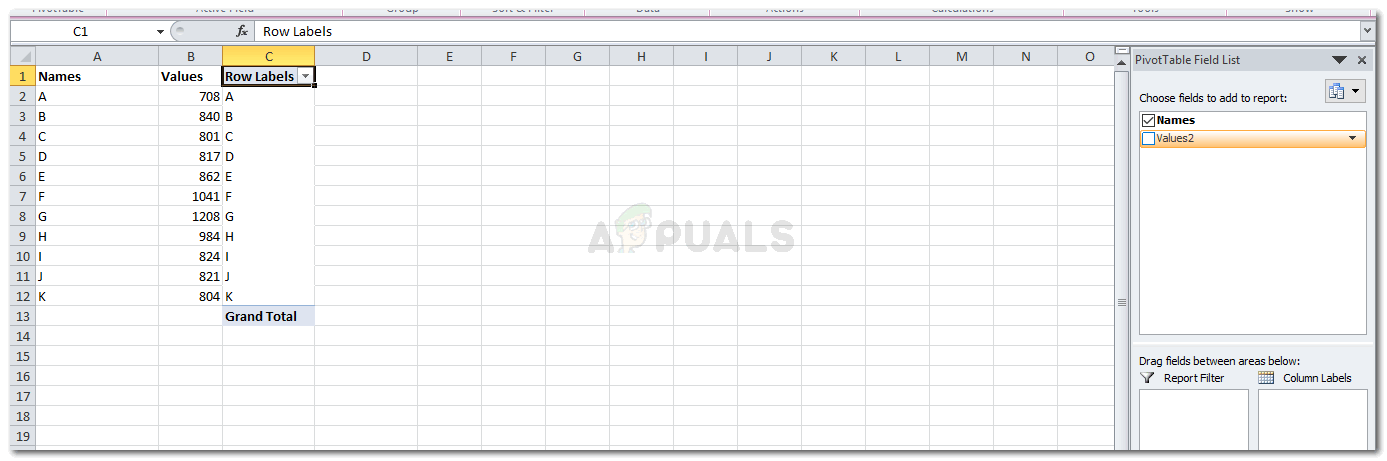
Displaying one field 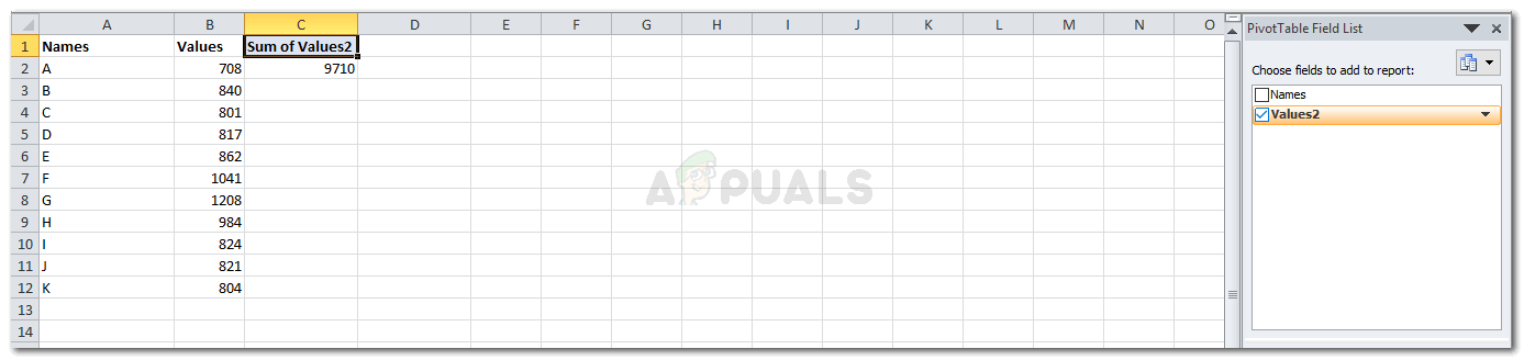
Displaying one field - The option on the right of your screen as shown in the picture below are very important for your report. It helps you make your report even better and more organized. You can drag the columns and rows in between these four spaces to alter the way your report appears.
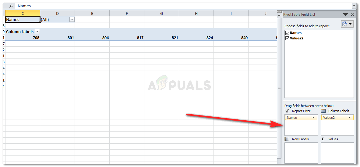
Important for placement of your report data 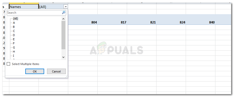
Your report has been made - The following tab on the Field list on your right makes your view of all the fields more easy. You can change it with this icon on the left.
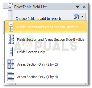
Options for the way your field view looks like. And choosing any of the options from these would change the way your field list shows. I selected ‘Areas Section Only 1 by 4’
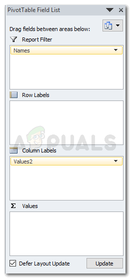
Field List view - Note: The option for ‘Defer Layout Update’ which is right at the end of your PivotTable Field List,is a way of finalizing the fields that you want displaying on your report. When you check the box next to it and click on update, you cannot change anything manually on the excel sheet. You will have to un-check that box to edit anything on the Excel. And even for opening the downward arrow showing on the columns labels cannot be clicked on unless you un-check the Defer Layout Update.
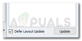
‘Defer Layout Update’, acts more like a lock to keep your edits to the content of the report untouched - Once you are done with your PivotTable, you can now edit it further by using the PivotTable Tools which appear right at the end of all the tools on your tool bar on the top.
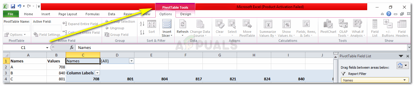
PivotTable Tools for editing how it looks 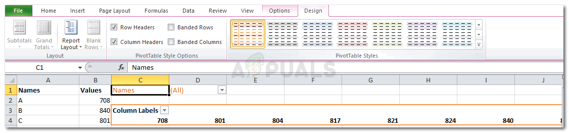
All the options for Design