Fix: “Formula Parse Error” with Examples on Google Sheets?
Encountering a parse error on Google Sheets is quite common for newbies as well as for experienced professionals. It is the way of the Sheets to tell you that there is something not right with your formula and Sheet cannot process the instructions given in the formula. These parse errors could be quite frustrating as you are expecting a calculated result but are “greeted” with the parse error, especially, if the error is occurring in a lengthy formula and the cause of the parsing error is not apparent.
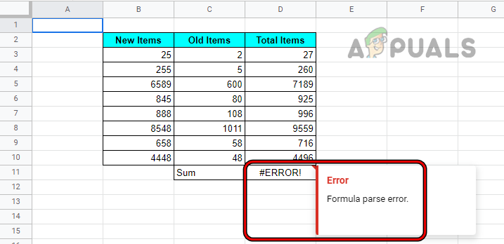
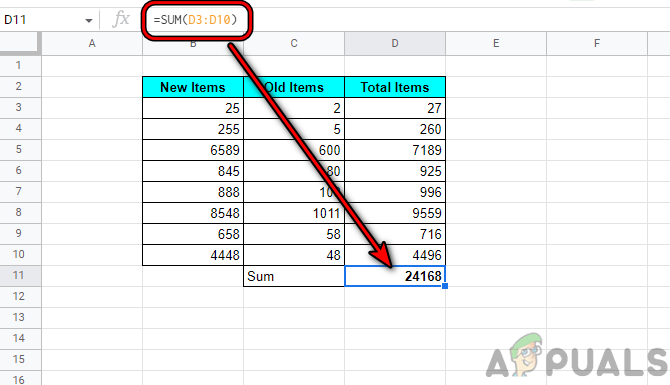
Once the Sheets show a parse error, it is simply telling you to correct your formula, arguments, data types, or parameters. A formula parse error is not a single error, there are many other errors under its hood like #N/A error, #error, etc. The parse error does not directly show in a wrong formula, it shows an error (like #error) but when you click on the error, then, in the side dropdown, it says formula parse error as shown in the image below where #Error! Is occurring in cell D11 but when clicked, it shows a formula parse error.
Google Sheets does not have a compiler (usually, linked to a parse error in the computing world). When a formula is entered in a Google Sheet, Sheets breaks down the syntax of the formula to analyze, categorize, and understand the syntax by using the parsing function. The parsing process consists of text dissection and the text is converted into tokens.
The Sheets parser function will then build a structure based on these tokens and other data received. If Sheets fail to perform the above on any of the formulae, then it will return a parse error. In simple words, parsing is dividing a large structure into smaller logical units for easier data storage and manipulation. Then Sheets re-compiles these as per the instructions and if any of these fail, that may lead to the Formula parse error.
Common Reasons for a Parse Error on a Google Sheet
The following are common reasons for which you may encounter a parse error:
- There is a typo in your formula like forgetting to put quote marks around a text string, putting two Sheets operators next to each other without anything to separate them. Also, an incomplete syntax (e.g., a missing parenthesis at the end of the formula) can cause a formula parse error.
- You have entered too few arguments or too many arguments as per the function’s requirements.
- The data types of the parameters of the formula are different from what Sheets is expecting like performing an addition operation on a text string will result in a parse error.
- The formula is trying to do an impossible mathematical operation (like dividing a value by zero or an empty cell).
- The formula is referring to an invalid cell range or the file you are referring to does not exist or is not accessible.
Types of Formula Parse Errors on a Google Sheet
The following are the most common types of parse errors on Google Sheets.
- There was a Problem Pop Up: When you encounter this type of error on Google Sheets, it means that the formula you entered is incorrect like adding a / at the end of the formula where it is not required.
- #N/A Error: This error means that your item was not found. Simply, the formula is searching for an item that does not present in the data.
- #Div/0 Error: This error means that you are trying to divide a value by zero. It implies that the formula calculations involve a step where the value is divided by zero, which is mathematically impossible.
- #Ref Error: This error means that your reference no longer exists. We can apprehend that the cells, files, links, images, etc. that the formula is referring to do not exist or is not accessible.
- #Value Error: This error means that your item is not of the expected type i.e., if you are adding two cells but one of the cells contains a text string, then the addition formula will return a #value error.
- #Name Error: This error means that you are incorrectly applying a label. For example, if you are using a named range in your formula, either you forget to add double quotes around it or the range name is not valid, then that would result in a #name error on a Google Sheet.
- #Num Error: If the result of a formula calculation is a very large number that cannot be displayed or is not valid, then that would result in a #num error on a Google Sheet like a square root of a negative number.
- #Null Error: This error means that the returned value is empty though it should not be. This error pertains to Microsoft Excel and is not a native error on Google Sheets. This error can only be cleared in Excel, not Google Sheets.
- #Error Error: If anything in your formula does not make sense to Google Sheets but Sheets are failing to point out the culprit (like a number issue by showing a #num error), then that could result in a #error. This type of error can sometimes become tough to troubleshoot as it is more generic, as all other ones are a bit specific. In other words, if an error does not fall in any other error types, Sheets will show #error for that error.
Fixes for a Parse Error on a Google Sheet
As we have covered the basics of the parse error, let us focus on troubleshooting it. But keep in mind that there is not a single size that fits all the scenarios and the troubleshooting process differs on a case-to-case basis. Let us discuss each error type with examples.
1. #N/A Error
This error is derived from the phrase “Not Available”. It mainly occurs in Lookup, HLookup, ImportXML, or similar functions which find a particular value in a given range. If that value is not available in the given range, then that would result in a #N/A error on a Google Sheet. Let us clarify the concept by the example.
- Look at the Google Sheet in the image below. It has data in cells B3 to B6, whereas, a N/A error is shown in cell D3.
- Then look at cell D3 and you will find the following Vlookup formula:
=VLOOKUP("Kiwis",B3:B6,1,0)
N/A Error in a VLOOKUP Formula - Now have a close look at the formula and you will notice that is it searching for Kiwis in the Fruits list but that list does not have Kiwis, thus the N/A error.
- Then you can clear the #N/A error either by adding Kiwis to the list or changing the formula to look for another value like Apples, as shown in the image below:

#N/A Error Removed After Changing the VLOOKUP Formula
You can use a similar approach to clear #N/A errors on your Google sheet.
2. #Div/0 Error
Divided by zero is donated as #Div/O in Google Sheets. If any step in your formula divides a value by zero or an empty cell, then that would result in a #Dive/0 error. Let’s clear it by the following example:
- A #/Div/0 error in the cell D3 in the sheet below which has 3 columns: Numbers, Divided by, and Result:
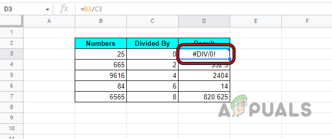
#Div Error on a Google Sheet - As the formula in D3 implies that the value in B3 (that is 25) should be divided by the value in C3 (that is zero), so, the formula is asking Google Sheets to perform 25/0, which is mathematically impossible, so the #Div error.
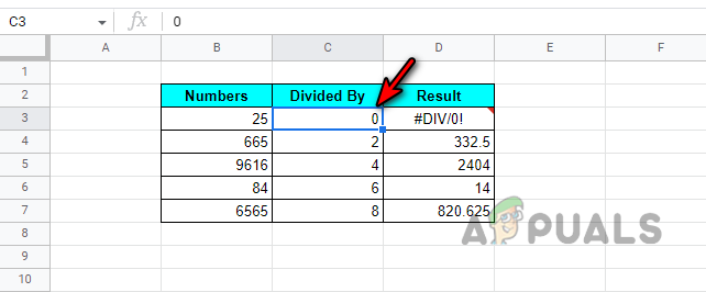
Divided By Zero Causing #Div Error - Now, this error can be cleared by removing zero from the divisor (here, cell C3) or if that is not possible, then either leave the formula as it is (if not used in another calculation) or mask the result by using the IFERROR function.
- In the given example, let us mask the #Div/0 as the Wrong Division by using IFERROR. The general syntax of IFERROR is as under:
=IFERROR(value, (value_if_error))
- In our example, the formula would be:
=IFERROR("Wrong Division",(B3/C3))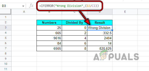
Use the IFERROR Function to Mask a N/A Error on A Google Sheet - Now you can see that the result in the D3 cell has changed to Wrong Division.
3. #Value Error
You may face a #value error on a Google sheet if the data type of at least a cell does not match what is required for the calculations to happen on a particular formula. In other words, a Google Sheet might show a #value error if you try to calculate a single data type (like a number) from two different input data types (like a number and a text string). Let us clear it by an example.
- Look at the sheet in the image below and you will notice a #value error the cell D3, although, other cells’ results are calculated correctly.
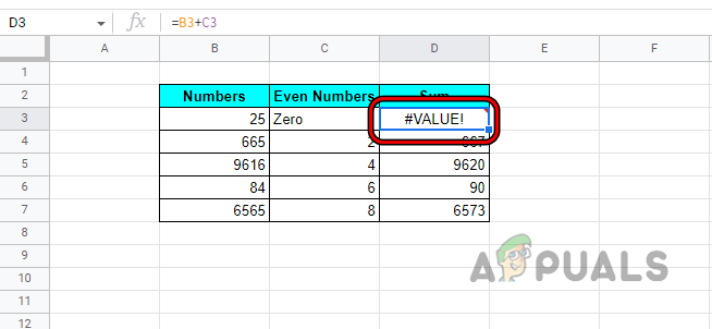
#Value Error on a Google Sheet - Then carefully inspect the formula and you will notice that cell D3 is a result of the addition of the value in cell B3 (that is 25) to the value of cell C3 (that is zero).
#Value Error Due to Summing a Text String with a Number - But zero is not a number but a text string, thus the Google Sheets fail to add a string to a number (different data types) and shows the #value error.
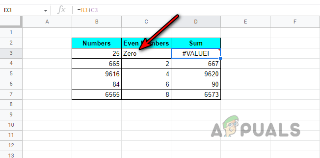
- Now, either you change the formula or change the value in the C3 cell from zero (text string) to 0 (numeric) as shown below:

Changing Zero Text to Numeric Zero Clears the #Value Error
4. #Name Error
A Google Sheet might show the #name error if a function name is misspelled, quotation marks are not present in the formula syntax (if required), or a cell/range name is not correct. We have a very detailed article on our website about #name errors, do not forget to check it.
- Reference to the sheet in the image below and you will notice a #name error in cell D3.
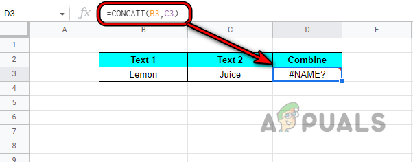
#Name Error on the Google Sheet - The D3 cell combines the values of B3 and C3.
- Our cell references (B3 and C3) are valid and do not have a typo, now have a good look at the formula in D3, you will notice that the formula is:
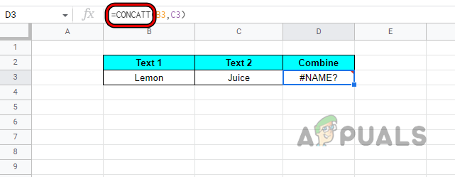
=CONCATT(B3,C3)
Concatt is Not a Valid Function of a Google Sheet - Whereas CONCATT (an extra T added to the correct CONCAT) is not a valid formula, it should have been:
=CONCAT(B3,C3)
- Now see the image below where the #name error is cleared after correcting the CONCAT formula.
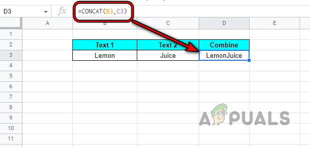
#Name Error Cleared After Correcting the Concat Formula
Let us take another example to clarify the idea about the #name error due to values.
- Reference to the sheet in the image below and you will notice a #name error in cell B3.
- Now have a good look at the formula and doesn’t everything look fine? Spellings of the CONCAT function are correct, lemon, and juice are also correct. Then what is causing the #name error?
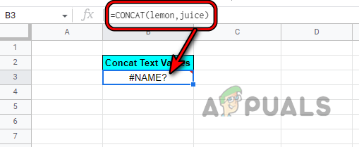
#Name Error Even Formula and Value are Correct - Lemon and juice are text strings and as per Google Sheets syntax, these should be wrapped in double quotes, as you can see in the image below that after adding quotes around lemon and juice, the #name error is cleared from cell B3.

#Name Error Cleared After Adding Double-Quotes Around the Text Strings
5. #Num Error
You may encounter the #num error on a Google sheet if the result of a calculation is larger than the maximum display capacity of Google Sheets i.e., 1.79769e+308. For example, if we multiply fifty-five billion by fourteen billion in a Google Sheet cell, then that will cause a #num error as Google Sheets cannot display such a large number. Another reason for this error is that the input type of a number does not meet the required type of the number type. Let us discuss it through an example:
- Refer to the sheet in the image below and you will notice a #num error in C7.

#Num Error on a Google Sheet - Now check the formula and you will notice that column C is the square root of column B.
- Then check cell B7 and you will find that it is a negative number but in basic mathematics, the square root of a positive number can be calculated only, thus Google Sheets throw a #name error.
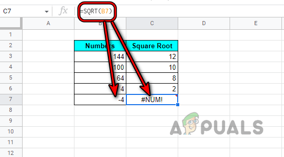
Square Root of A Negative Number Causing the #Num Error on A Google Sheet - You can correct this either by changing the value (you can use the ABS function to convert the number to positive), formula, or hiding the result by using IFERROR (as discussed earlier).
6. “#Error” Error
If a Google Sheet cannot understand a particular formula but cannot specify the reason for the error (like other errors where we get a hint like in #num error we know that the problem is with numbers), then that could result in a “#error” error. As the reason for the error is not specified, it is a more general error in nature or we can say that if a Google Sheet cannot link an error to any other error types of the parse error, then it will show a “#error” error. It could be a result of missing characters like commas, apostrophes, values, and parameters. Let us understand it with the following example:
- Look at the sheet in the image below and you will notice a “#error error” in cell D11.
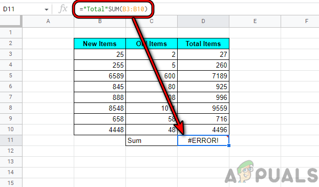
- Now have a good look at the formula in D11 and you will notice it is as under (as we are trying to sum the sums):
="Total"SUM(B3:B10)

A Wrong Sum Formula Caused #Error Error on a Google Sheet - But the total sum is not a valid function and we will only need a Sum Function to sum the sums like:
=SUM(B3:B10)
- Now check the sheet below after making the above amendment that clears the #error error:
#Error Cleared After Correcting the SUM Formula in a Google Sheet
As this error is general, here are some steps that you may take to clear this type of parse error:
- Make sure the opening and closing parentheses in a formula match according to the amount required.
- If special characters such as the colons, semicolons, commas, and apostrophes are placed properly (if required by the formula).
- If the data contains dollar or percentage signs, make sure they are not part of your formula. Ensure those are input as normal numbers. If you are in a requirement to use these signs, then format the results as currencies (like Dollar) or percentages, not the inputs.
7. #Ref Error
This error might occur on a Google Sheet if the cell references used in the formula are not valid or missing. This error can mainly occur due to the followings:
- Deleted Cell References
- Circular Dependency
- Cell Reference Out of the Data Range
#Ref Error Due to Deleted Cell References
If a formula is referring to a cell range but that cell range is deleted, then it will cause a #ref error in the formula cell. Let us discuss an example in this regard:
- Refer to the image below and you will see a Sum column is set up in cells D3 to D7 that is adding columns B and C.

Sum Formula in the D Column - Now, we delete column C and that will cause a #ref error in column D as column C is deleted, which is part of the formula, thus #ref error.
#Ref Error After Deleting a Column on a Google Sheet - Here, either un-delete column C or amend the formula to remove references to deleted cells.
#Ref Error Due to Circular Dependency
If a formula cell is referring to itself as an input range, then that will cause a #ref error due to circular dependency. Let us clarify the concept by the following example:
- Reference to the sheet in the image below and you will notice a #ref error in cell B11.
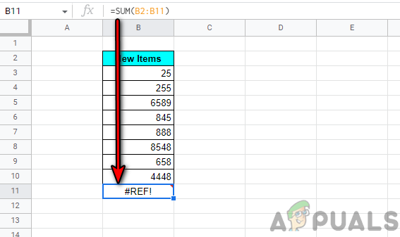
#Ref Error on a Google Sheet - Now look to the formula in the cell B11:
=SUM(B2:B11)

#Ref Error Due to Circular Dependency - Then you will notice that the B11 cell is also referred to in the range and is also an input cell to itself, so #ref error due to the circular dependency.
- In this case, edit the formula to remove the cell from the referred range which clears the #ref error from B11:
=SUM(B2:B10)

#Name Cleared After Removing the Circular Dependency in the Formula
#Ref Error Due to Cell Reference Out of the Data Range
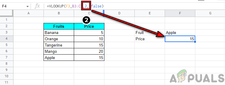
If you are using a function (like VLOOKUP) to search/extract an entry in a selected cell range but the cell reference given is outside the selected range, thus a #REF! error due to cell reference being out of the data range. Let’s discuss it through an example:
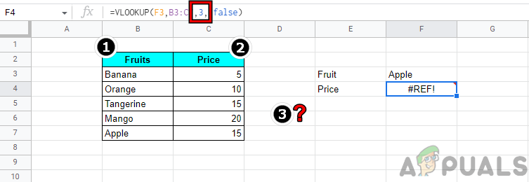
- Refer to the sheet shown in the image below and you will notice a #ref error in cell F4.

#Ref Error in the VLOOKUP Formula on A Google Sheet - Now look at the formula and you will find that it is referring to the 3rd column in the range (B3 to C7), whereas, the range has only two columns (B and C), thus #ref error due to cell reference out of the data range.
#Ref Error Due to Referring to a Column That is Not Present in the Range - Then edit the formula to use the 2nd column (the price column) and thus that clears the #ref error.
#Ref Error Due to Due to Cell Reference Out of the Data Range Cleared After Changing the Formula to Use Correct Column
8. There Was a Problem Pop Up
This is probably the most recurring type of parse error. When this error occurs, you cannot do anything on the sheet till you fix or skip the formula. This error mostly occurs if a character is missing from the formula’s syntax or an extra character is present in the formula syntax. You can understand it by the following example:
- Refer to the sheet displayed in the image below and you will notice that There Was a Problem Pop Up shown when adding a sum formula in the cell B11:
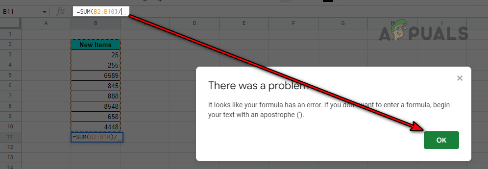
There Was a Problem Error on A Google Sheet - Now you will notice that there is an extra / at the end of the formula and thus causing the parse error under discussion.
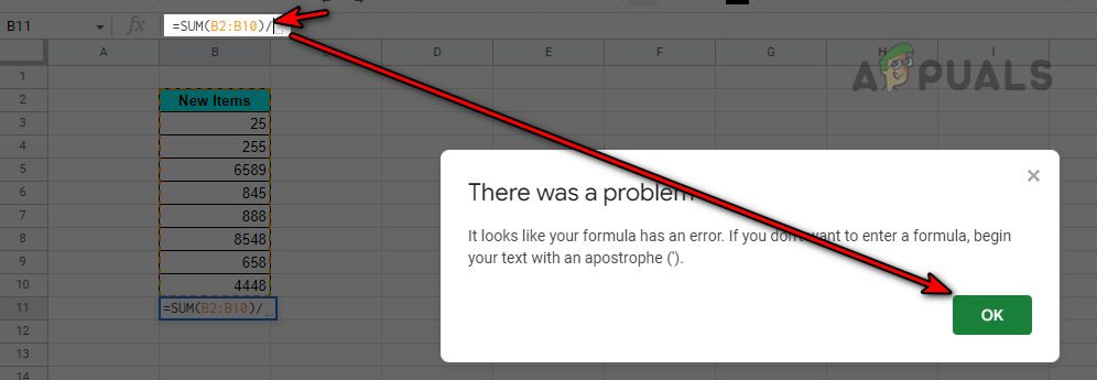
There Was a Problem Error on A Google Sheet - Then remove the / from the formula and that will clear the error:
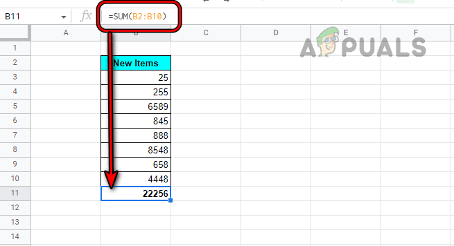
There Was a Problem Error Cleared on the Google Sheet After Removing Slash From the End of the Formula
9. #Null Error
This error mainly occurs in Excel and if you copy the data from an Excel sheet to a Google sheet, then that may show a #null error. If an Excel sheet is uploaded to Google Sheets, then that data may show the
#error” error, not the #null error. Then either you clear the #null error in Excel or clear the “#error” error on Google Sheets (discussed earlier).

Functions to Deal Errors on a Large Google Sheet
As the above examples were simple to make the idea clear but on a large sheet, it becomes troublesome to find and troubleshoot errors. We are listing down some Google Sheet functions that make this process easier.
ISNA Function
You can use this function to check the selected cell range for a N/A error. It uses the following syntax:
=ISNA(value)
ISERR Function
If you are interested in all others errors in a range except the #N/A error, then this function will list down all such errors. Following is the syntax of this function:
=ISERR(value)
The ERROR TYPE Function
This Google Sheets function lists down every error on a sheet in numbers. It takes the following syntax:
=ERROR.TYPE(value)
The errors detected and the corresponding numbers are as followings:
#NULL!=1

#DIV/0!=2

#Value=3

#Ref=4

#NAME?=5

#NUM!=6

#N/A!=7

All other random errors on a Google sheet=8
If Error Function
If a parse error cannot be rectified due to circumstances, then you may hide it by using the IFERROR function, if no other calculations are getting disturbed. Please use it as a last resort because it can cause unintended issues in the future. You can refer to the #Div/0 Error section to understand the process.
Best Practices to Avoid a Parse Error
It is always better to avoid an error than to waste countless hours troubleshooting it. Here are some of the best practices that you can use to avoid parse errors.
- Make sure not to use symbols like % or $ in a formula.
- Punctuation marks in a formula are changed as per your region and language in a Google Sheet, so, if you are facing a parse error in a Google sheet, you may switch between commas to semicolons or vice versa to clear the error. In some regions, you may have to use \ instead of commas or semicolons.
- Keep in mind that you must write a formula in Google Sheets in English, even If you are using Google Sheets in a non-English language like French.
- Make sure your Locale in Spreadsheet Settings of Google Sheets and Time Zone are set to the same place as the United States, not like Locale set to the United States, and Time Zone set to Moscow.
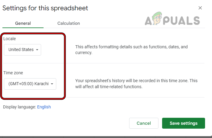
Set Locale and Time Zone of A Google Sheet to the Same Place - If a parse error occurs on a Google Sheet, do not forget to check for the placement of quotes around text, links, image sources, etc. Also, keep an eye on when to use single quotes and when to use double quotes.
- When referring to a cell in another sheet in a formula, make sure to select the required cell on that sheet, not type it as it can sometimes return a parse error.
- Do note that when a plus sign and comma are used in a formula (this can happen when dealing with phone numbers) like the following, it will return a parse error on a Google Sheet.
+123,456                     // This will result in an error

+123456                      // This will not result in an error
- When copying or referring to whole columns or rows on a sheet from another sheet, always start with the 1st column or row, otherwise, mismatching rows and columns between the source and destination sheets will cause a parse error.
- Last, but not least, here is the link to a Google Sheet (without any Macros, add-ons, etc. but you must copy the sheet to your Google Sheets). This is an automated tool built as Evaluate Formula Parser (Google Sheets does not have one, whereas, Excel is equipped with it). This sheet can be used to evaluate a formula that is showing a parse error. You must use this sheet at your own risk and we will not be responsible for any issues caused by this sheet.
Hopefully, we have succeeded in clearing the parse errors on your Google sheet. If you have any queries or suggestions, you are more than welcome in the comments section.