How To Unhide Columns in Microsoft Excel [5 Easy Ways]

Among the plethora of features you get with Microsoft Excel, the ability to hide and unhide columns can often go unnoticed. This unique feature allows spreadsheet creators to make viewers focus on certain key figures and safeguard sensitive information from everyone.

With this in mind, if you are working with Excel files with hidden columns, it’s important to learn how to unhide columns in Excel to extract maximum data. So get your spreadsheets ready and let’s jump in!

How Does Hiding Columns Work in Excel?

Including data points for calculations and summaries is common when working on Excel. While all that is important, you don’t want your viewers to see that mess. That is where hidden columns come in handy.

This feature allows you to hide information such as formulas from your view while keeping it in the spreadsheet. Hiding columns makes your spreadsheet easy to understand and enhances its overall aesthetics.

READ MORE: How to Hide Columns in Excel – 6 Ways With Easy Steps ➜

How to Identify Hidden Columns

One of the easiest ways to identify hidden columns is by looking for a double line or a gap between the top column headers. Another way to identify hidden columns is by checking for missing column letters. This gives users a visual cue that some of the columns are hidden.

5 Ways to Unhide Columns in Excel

When bringing back hidden columns to your spreadsheet, you have 5 different ways to help you get the job done. Let’s break all of them down individually:

1. Unhide Columns in Excel Using the Context Menu

This method allows you to reveal hidden columns directly from the context menu. Here’s a quick rundown to unhide columns using the context menu:

1. First, identify the hidden columns you want to reveal.
   

   

2. Once that’s done, select the two adjacent columns near your hidden columns. For instance, if Column G is hidden, select Columns F and H.
   

   

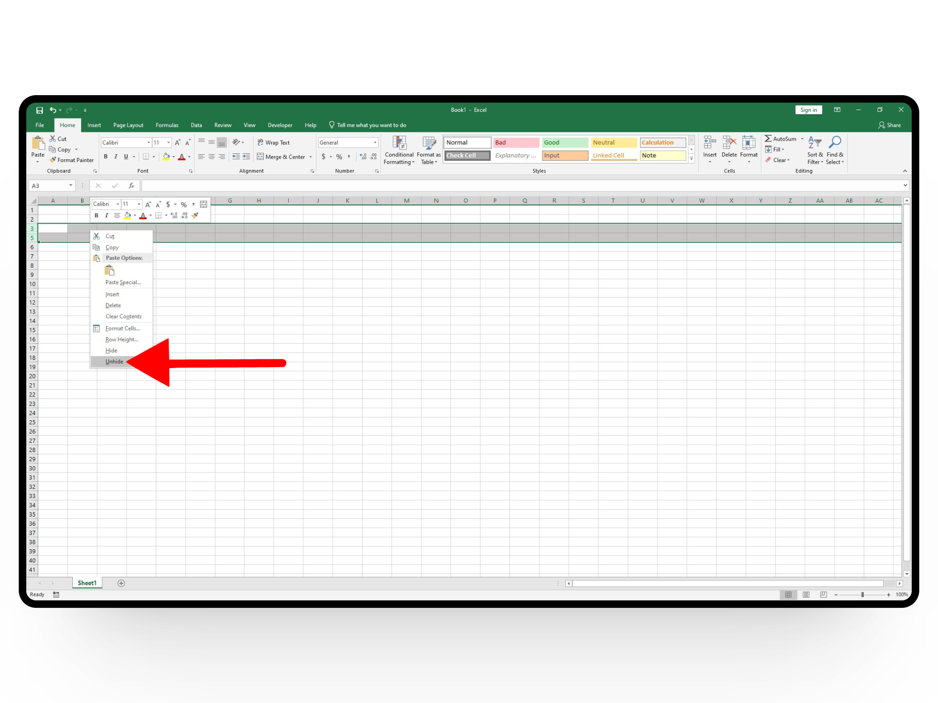
3. Next, right-click on one of the column headers. This will open up the Context Menu. Here, select the Unhide option.
   

   

4. The hidden column should appear in between the two selected columns.
   

   

READ MORE: How to Get Dark Mode in Google Sheets – Desktop & Mobile ➜

2. Unhide Columns in Excel Using Keyboard Shortcuts

Another quick way to unhide columns in Excel is by using keyboard shortcuts allowing you to save the time and effort of manually going through different tabs and sections. When using shortcuts, you have two options that offer the same purpose:

• ALT + H + O + U + L
• ALT + O + C + U

Apart from a few different keys, both these combinations serve the same purpose and will reveal all hidden columns from your spreadsheet.

READ MORE: How to Fix Keyboard Automatically Doing Shortcuts While Typing? ➜

3. Unhide Columns in Excel Using the Ribbon

The second method to unhide columns in Excel is by using the Ribbon menu which also refers to the tools at the top of your page that help manage your data. Here’s how that’s done:

1. Select the adjacent columns next to your hidden columns.
   

   

2. From here, head over to the Home tab and click on the Format option in the Cells section.
   

   

3. From the drop-down menu, head to the Visibility section and hover over to the Hide & Unhide tab.
   

   

4. Next, click on the Unhide Columns to reveal hidden columns on your sheet.
   

   

READ MORE: 3 Ways to Open Microsoft Excel in Safe Mode ➜

4. Unhide Columns in Excel Using Width Increase

This method isn’t one of the most conventional ways to unhide columns and is often used by beginners as it takes up a lot of time when manually doing it. However, it’s good to have it in your mind when working with someone who doesn’t know Excel adequately.

1. Identify the hidden column from the gap lines.
   

   

2. Next, hover over to the rightmost line and drag it while pressing and holding the mouse button. 
   

   

3. As and when you do this, the hidden column should slowly start appearing. Release the mouse button when it’s properly visible.
   

   

READ MORE: VLOOKUP vs XLOOKUP: Which is the better Excel Formula? ➜

5. Unhide Columns Using Excel VBA

Excel VBA (Virtual Basic for Applications) is a great way to automate tasks and customize certain operations. However, to use this method properly, you will need to have a basic grip on applying VBA codes. Here’s how to unhide columns using Excel VBA:

1. Head over to the Developer tab from the ribbon and click on the Visual Basic option. 
   

   

2. Once the application opens up, click on the Insert tab and select the Module option. 
   

   

3. Here, you’ll have the option to type in the following commands:

If you want to unhide a specific column, type in this command:

Sub Unhide_Columns()
Columns("B:B").Hidden = False
End Sub

If you want to unhide a range of columns, type in this command:

Sub Unhide_Columns()
Columns("B:D").Hidden = False
End Sub

And that’s pretty much it. While using VBS is good for automating even the most complex tasks, we don’t suggest it for unhiding columns considering you have easier alternatives at hand.

If you don’t have the Developer option on your Ribbon, you’ll need to open Options > Customize Ribbon and check the Developer box under Main tabs.

READ MORE: How to Switch Between Sheets and Cells on Microsoft Excel ➜

How to Unhide Column A in Excel (First Column)

When working on spreadsheets with a hidden first column, it can be tricky to unhide it as there’s no manual way to select the A column as you can with others. To work around that, here’s how to unhide column A in Excel:

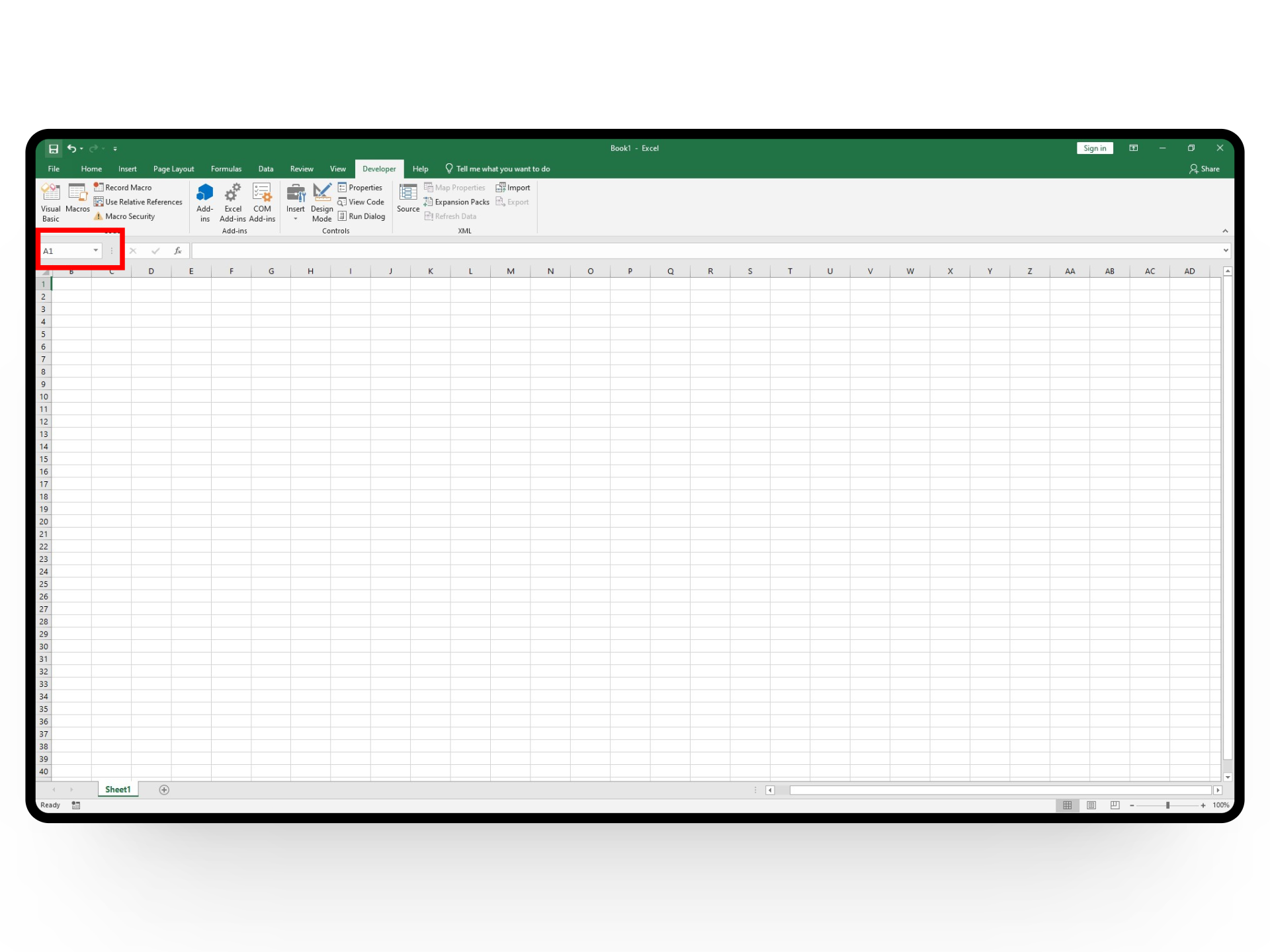
1. Click on the Name Box in the top left corner of your document.
   

   

2. Next, type in “A1” or any other cell name from the A column. Excel will select your cell, but you won’t be able to see the usual green box around it.
   

   

3. Next, head over to the Format tab and click on the Unhide Columns button under the Visibility section.
   

   

Additionally, you can also try increasing the width of the first column by dragging the line to unhide it and bring it to your view.

READ MORE: How To Solve #Div/0 Errors in Excel (with Examples) ➜

Bonus: How to Unhide Rows in Excel

Just like hidden columns, hidden rows can also be identified by a double-line marker between rows. Additionally, you will also see row number labels skip the usual numerical order and appear randomly. Once you have your hidden rows identified, follow these steps:

1. Select the top and bottom rows that are adjacent to your hidden row. 
   

   

2. Next, right-click anywhere in the selection and select Unhide from the Context menu.
   

   

While this is the most basic and simplest way to do it, you can also try out the above-mentioned steps to unhide columns and they will work the same way for hiding rows.

READ MORE: How to Calculate Standard Error in Excel? ➜

Bonus: How to Unhide Row 1 in Excel (First Row)

Similar to the A column, you can also unhide the first row to reveal important information regarding column headers. Here’s how to unhide the first row in Excel:

1. Click on the Name Box at the top left corner of your document.
   

   

2. Here, type in the cell name such as A1.
   

   

3. Finally, head over to the Format tab and click on the Unhide Rows option from the Visibility tab.
   

   

READ MORE: How to Fix #Name Error in Excel (with Examples) ➜

Unhide All Columns and Rows in Excel

If your spreadsheet has several hidden columns and rows, manually unhiding them through different methods can be a hassle. However, you can make things convenient by selecting the entire spreadsheet to unhide all columns and rows.

To carry it out all you need to do is first select the entire spreadsheet by clicking on the small grey downward-facing triangle at the top left corner of your screen. Once it turns green, right-click anywhere on the column header and select the Unhide option from the context menu.

READ MORE: How to Make a Line Graph in Google Sheets [2024] ➜

Disable the Option to Unhide Columns in Excel

If you don’t want users to unhide hidden columns, Excel also gives you the option to protect your sheet from others accessing sensitive data. With this setting enabled, anyone (including you) will not be able to unhide columns and you’ll have to enter a password to make these options accessible again.

Here’s how to disable the option to unhide columns in Excel:

1. Select the entire sheet by clicking on the grey triangle icon. 
   

   

2. Next, right-click anywhere on the column headers to open up the context menu. Here, select the Format Cells option.
   

   

3. From here, head over to the Protection tab > uncheck the Locked option and hit OK.
   

   

4. Now, select the columns you want to hide and once again head to the Format Cells option but this time check the Locked box. 
   

   

5. Next, head over to the Review tab and click on the Protect Sheet option.
   

   

6. From the menu, make sure the Select locked cells and Selected unlocked cells are checked. Now type in a password of your choice and hit OK after confirming it.
   

   

7. And that’s it. The Unhide option should now be disabled for everyone.
   

   

To enable the option back again, simply click on the Unprotect Sheet option and enter your password.

READ MORE: What’s the ROUNDDOWN Function? How to use it?

Find Any Hidden Rows and Columns in the Workbook

Another interesting feature that comes with Excel is the built-in Workbook tool that allows users to inspect a document for all hidden rows and columns.

Here’s how to find any hidden rows and columns in the workbook:

1. Click on the File option in the top left corner.
   

   

2. From here, select the Info option from the sidebar and click on the Inspect Workbook option.
   

   

3. This will open a small drop-down menu. Here, click on the Inspect Document option to open up the Document Inspector.
   

   

4. Here, you’ll have the option to check any specific detail. Scroll down and select the Hidden Rows and Columns tab.
   

   

5. As and when you click on the Inspect button, Excel will prompt you with the number of all hidden rows and columns along with the option to Remove All. 
   

   

Alternative to Hiding and Unhiding Columns — Grouping

In Microsoft Excel, Hiding columns and Grouping them are two different features with different purposes. Hiding columns allows you to make certain information invisible without deleting it. On the other hand, Grouping organizes your data into collapsible sections making them useful for creating a structured and navigable layout for sheets with large datasets.

Additionally, hidden columns are hard to spot when quickly scrolling through a spreadsheet, whereas Grouping is much more distinct with a bold line above the grouped section that can be expanded or collapsed with just a click.

To use the grouping feature all you have to do is select your columns and either use the shortcut keys “ALT + SHIFT + Right Arrow” or head to the Data Ribbon and use the Group and Ungroup options. After grouping columns in Excel, you can expand or collapse the grouped section by clicking the “+” or “–” icon.

READ MORE: How to Password Protect or Encrypt Excel Files ➜

Conclusion

To unhide columns in Excel, you have several different ways to get the job done. Once you master this feature you can not only improve the quality of your sheets but also protect data. Additionally, if you want to make enhance your content’s visibility, you can also try using the Grouping alternative to add collapsible sections to your project.